![]()
fixes is an R package for event study
analysis in panel data — the workhorse tool for visualizing
parallel trends and dynamic treatment effects in
difference-in-differences research.
Version 0.8.0 adds three modern estimators designed for
staggered adoption (where different units adopt
treatment at different times), all accessible through the same
run_es() interface.
Key functions:
| Function | What it does |
|---|---|
run_es() |
Estimate an event study (4 estimators available) |
plot_es() |
Static ggplot2 event study plot |
plot_att_gt() |
Visualize the full ATT(g,t) matrix (CS estimator) |
plot_es_interactive() |
Interactive plotly plot with hover tooltips |
Estimators (selected via the estimator
argument in run_es()):
estimator |
Reference | Best for |
|---|---|---|
"twfe" |
Classic TWFE | Universal treatment timing |
"cs" |
Callaway & Sant’Anna (2021) | Staggered adoption |
"sa" |
Sun & Abraham (2021) | Staggered adoption |
"bjs" |
Borusyak, Jaravel & Spiess (2024) | Staggered adoption |
# From CRAN
install.packages("fixes")

# Development version
pak::pak("yo5uke/fixes")library(fixes)All four estimators share the same interface:
# Classic TWFE (single treatment date)
res_twfe <- run_es(
  data = df,
  outcome = y,
  treatment = treat,
  time = period,
  timing = 5,
  fe = ~ id + period
)

# Sun & Abraham (2021) — staggered adoption
res_sa <- run_es(
  data = df_stagg,
  outcome = y,
  time = year,
  timing = timing,
  unit = id,
  fe = ~ id + year,
  staggered = TRUE,
  estimator = "sa"
)

# Callaway & Sant'Anna (2021) — staggered adoption
res_cs <- run_es(
  data = df_stagg,
  outcome = y,
  time = year,
  timing = timing,
  unit = id,
  staggered = TRUE,
  estimator = "cs",
  control_group = "nevertreated"
)

# Borusyak, Jaravel & Spiess (2024) — staggered adoption
res_bjs <- run_es(
  data = df_stagg,
  outcome = y,
  time = year,
  timing = timing,
  unit = id,
  staggered = TRUE,
  estimator = "bjs"
)Use run_es() with a fixed event date. Here we use
fixest::base_did, a simulated balanced panel where all
units are treated at period 5.
df <- fixest::base_did

es <- run_es(
  data = df,
  outcome = y, # outcome variable (unquoted)
  treatment = treat, # 0/1 treatment indicator
  time = period, # time variable
  timing = 5, # treatment occurs at period 5
  fe = ~ id + period,
  cluster = ~id,
  baseline = -1 # period -1 is the reference (default)
)

print(es)
## Event Study Result (fixes)
## N: 1080 | Units: NA | Treated units: 1080 | Never-treated: NA
## FE: id + period
## VCOV: HC1 | Cluster: id
## Method: classic | lead_range: 4 lag_range: 5 baseline: -1plot_es(es)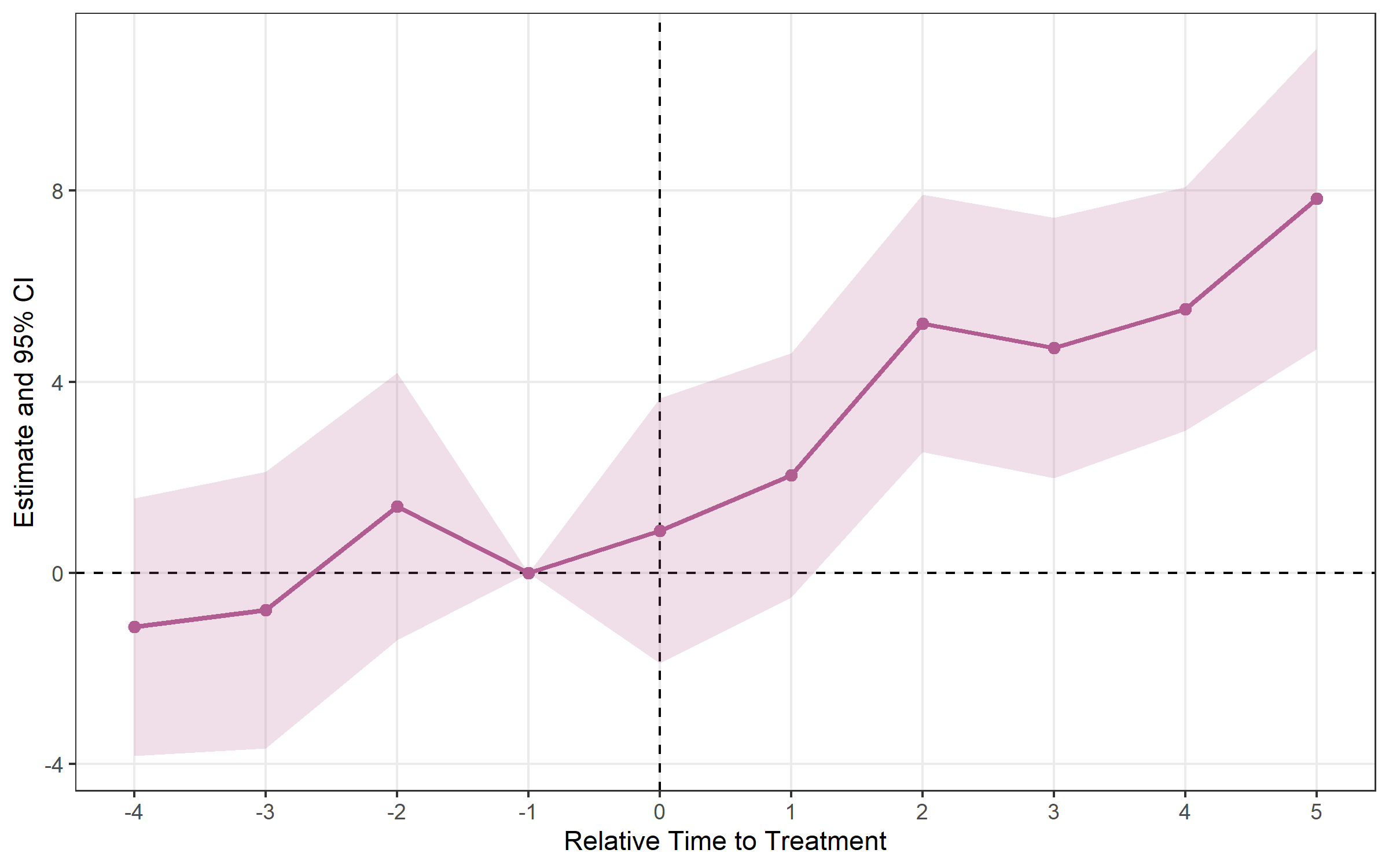
When units adopt treatment at different times, the classic TWFE
estimator can be biased. fixes provides three modern
alternatives.
Setup: create a shared dataset from
fixest::base_stagg. Never-treated units use NA
for their timing column — this is the convention for all three staggered
estimators.
df_stagg <- fixest::base_stagg
df_stagg$timing <- df_stagg$year_treated
df_stagg$timing[df_stagg$year_treated == 10000] <- NA # mark never-treatedestimator = "cs"Estimates a separate ATT(g,t) for every combination of cohort g and calendar time t, then aggregates to the event-study curve. Comparison group can be never-treated units (default) or not-yet-treated units.
cs <- run_es(
  data = df_stagg,
  outcome = y,
  time = year,
  timing = timing, # first treatment period; NA = never treated
  unit = id,
  staggered = TRUE,
  estimator = "cs",
  control_group = "nevertreated" # or "notyettreated"
)

print(cs)
## Event Study Result (fixes)
## N: 950 | Units: 95 | Treated units: 45 | Never-treated: 50
## FE:
## VCOV: analytic | Cluster: -
## Method: classic | lead_range: 9 lag_range: 8 baseline: -1plot_es(cs)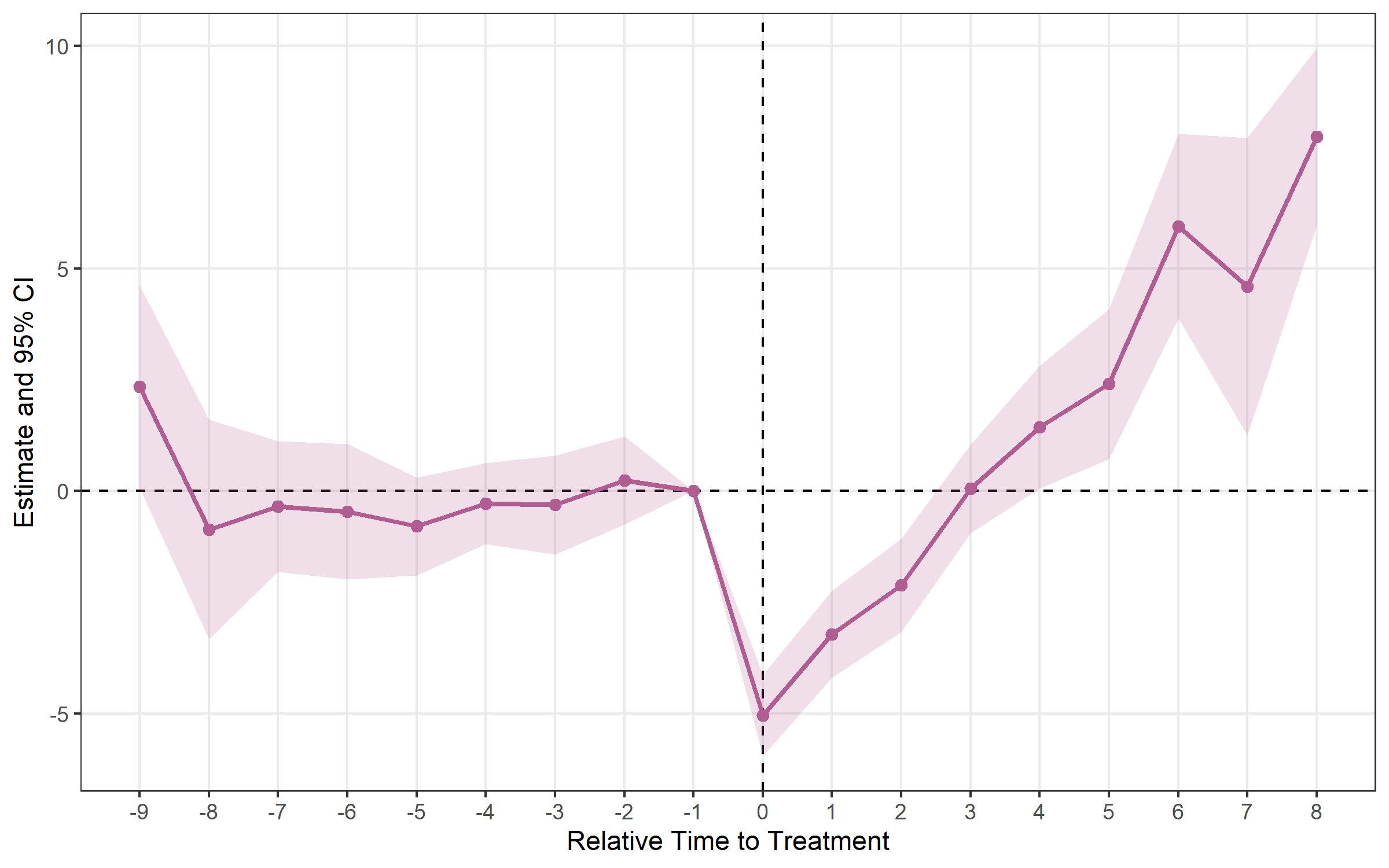
plot_att_gt() shows every cohort × calendar-time cell,
making it easy to spot anticipation effects or heterogeneous
dynamics.
plot_att_gt(cs, type = "heatmap")
plot_att_gt(cs, type = "facet")
estimator = "sa"Builds cohort × horizon interaction terms, then aggregates with
cohort-share weights. Gives the same result as
fixest::sunab() but through the unified
run_es() interface.
sa <- run_es(
  data = df_stagg,
  outcome = y,
  treatment = treated,
  time = year,
  timing = timing,
  unit = id,
  fe = ~ id + year,
  staggered = TRUE,
  estimator = "sa",
  cluster = ~id
)

print(sa)
## Event Study Result (fixes)
## N: 950 | Units: 95 | Treated units: 45 | Never-treated: 50
## FE: id + year
## VCOV: HC1 | Cluster: id
## Method: classic | lead_range: 9 lag_range: 8 baseline: -1plot_es(sa)
estimator = "bjs"A three-step imputation approach:
bjs <- run_es(
  data = df_stagg,
  outcome = y,
  time = year,
  timing = timing,
  unit = id,
  staggered = TRUE,
  estimator = "bjs"
)

print(bjs)
## Event Study Result (fixes)
## N: 950 | Units: 95 | Treated units: 45 | Never-treated: 50
## FE: id + year
## VCOV: bjs_conservative | Cluster: -
## Method: classic | lead_range: 1 lag_range: 8 baseline: -1plot_es(bjs)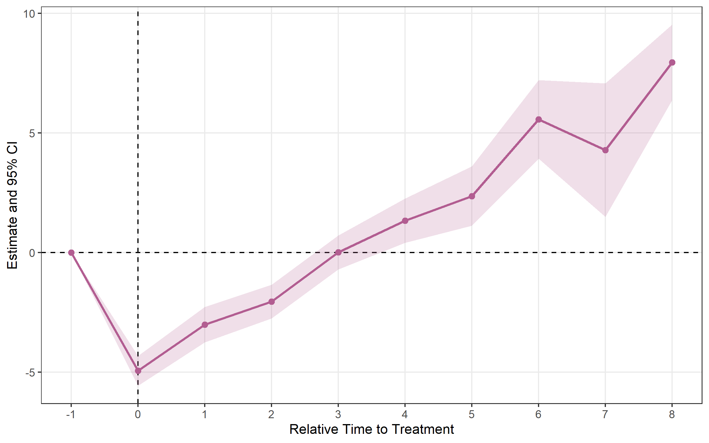
Pointwise confidence intervals control error rates one period at a time. When you display 15 pre- and post-treatment estimates on a single plot, the chance that at least one interval incorrectly excludes zero can be much higher than the nominal 5%.
Simultaneous bands (Callaway & Sant’Anna 2021, Corollary 1) provide joint coverage: with probability ≥ 1 − α, the entire event-study curve is contained within the band.
Use bootstrap = TRUE in run_es() and
show_simultaneous = TRUE in plot_es():
cs_boot <- run_es(
  data = df_stagg,
  outcome = y,
  time = year,
  timing = timing,
  unit = id,
  staggered = TRUE,
  estimator = "cs",
  control_group = "nevertreated",
  bootstrap = TRUE, # run multiplier bootstrap (Algorithm 1, CS 2021)
  B = 999, # number of bootstrap draws; 999 recommended in practice
  boot_seed = 42 # for reproducibility
)
# Lighter outer band = simultaneous CI; darker inner band = pointwise CI
plot_es(cs_boot, show_simultaneous = TRUE)The simultaneous band is always at least as wide as the pointwise band. The interactive plot also gains a second ribbon trace:
plot_es_interactive(cs_boot, show_simultaneous = TRUE)plot_es() works with results from any estimator.
# Error bars instead of ribbon
plot_es(es, type = "errorbar")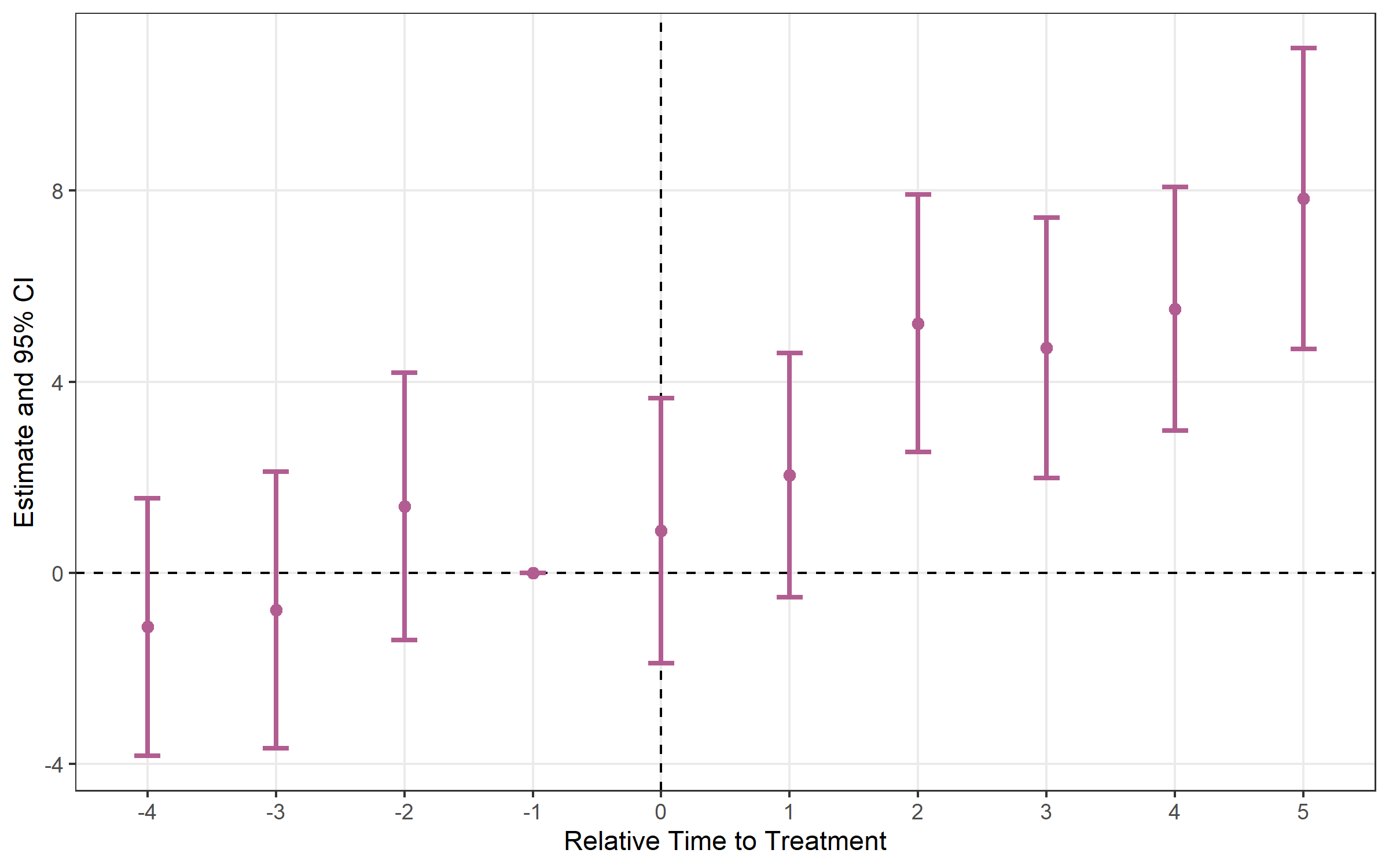
# Multiple CI levels at once
es_multi <- run_es(
  data = df,
  outcome = y,
  treatment = treat,
  time = period,
  timing = 5,
  fe = ~ id + period,
  cluster = ~id,
  conf.level = c(0.90, 0.95, 0.99)
)
plot_es(es_multi, ci_level = 0.90, theme_style = "minimal")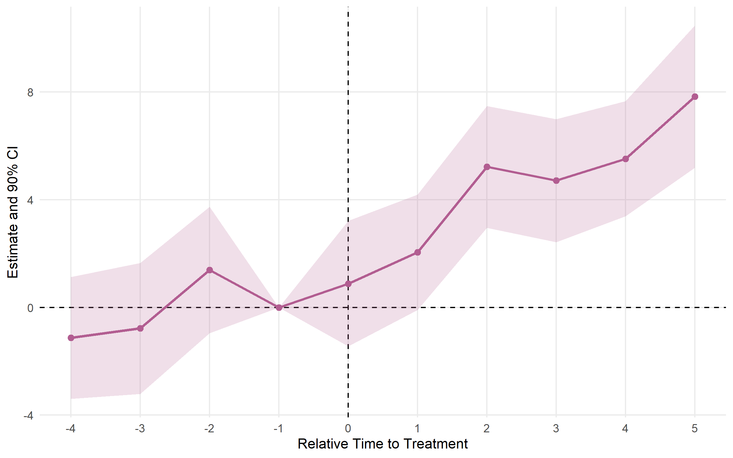
plot_es_interactive() produces a plotly chart with hover
tooltips (requires the plotly package).
plot_es_interactive(es)run_es() arguments| Argument | Default | Description |
|---|---|---|
data |
— | Panel data frame |
outcome |
— | Outcome variable (unquoted) |
treatment |
NULL |
0/1 treatment dummy ("twfe" only) |
time |
— | Time variable (numeric) |
timing |
— | Treatment date (scalar for "twfe", column for others;
NA = never treated) |
unit |
NULL |
Unit ID column (required for "cs", "sa",
"bjs") |
fe |
NULL |
Fixed effects formula, e.g. ~ id + year |
estimator |
"twfe" |
"twfe", "cs", "sa", or
"bjs" |
staggered |
FALSE |
Set TRUE for unit-varying treatment timing |
control_group |
"nevertreated" |
CS only: "nevertreated" or
"notyettreated" |
cluster |
NULL |
Clustering formula, e.g. ~ id |
baseline |
-1 |
Reference period (0 = treatment date) |
lead_range |
auto | Pre-treatment periods to show |
lag_range |
auto | Post-treatment periods to show |
conf.level |
0.95 |
CI level(s); vector allowed, e.g. c(0.90, 0.95) |
vcov |
"HC1" |
VCOV type (any fixest::vcov() type) |
bootstrap |
FALSE |
CS only: run multiplier bootstrap for simultaneous CIs |
B |
999 |
CS bootstrap: number of draws |
boot_seed |
NULL |
CS bootstrap: RNG seed for reproducibility |
Found a bug or have a feature request? Open an issue on GitHub.