![]()
![]()

paleopop is part of the poemsverse. poems
is a spatially-explicit, process-explicit, pattern-oriented framework
for modeling population dynamics. This extension adds functionality for
modeling large populations at generational time-steps over
paleontological time-scales.
You can install the latest release of paleopop from CRAN
with:
install.packages("paleopop")
#> Installing package into '/home/runner/work/_temp/Library'
#> (as 'lib' is unspecified)
You can install the development version from GitHub with:
# install.packages("devtools")
devtools::install_github("GlobalEcologyLab/paleopop")poems and paleopop are based on R6 class objects. R is primarily a
functional programming language; if you want to simulate a
population, you might use the lapply or
replicate functions to repeat a generative function like
rnorm. R6 creates an object-oriented programming
language inside of R, so instead of using functions on other functions,
in these packages we simulate populations using methods attached to
objects. Think of R6 objects like machines, and methods like switches
you can flip on the machines.
One of the major additions in paleopop is the
PaleoRegion R6 class, which allows for regions that change
over time due to ice sheets, sea level, bathymetry, and so on. The plots
below show the temporal mask functionality of the
PaleoRegion object. The temporal mask indicates cells that
are occupiable at each time step with a 1 and unoccupiable cells with a
NA. In this example, I use the
temporal_mask_raster method to show how “Ring Island”
changes at time step 10 due to a drop in sea level.
library(poems)
library(paleopop)
coordinates <- data.frame(x = rep(seq(-178.02, -178.06, -0.01), 5),
                          y = rep(seq(19.02, 19.06, 0.01), each = 5),
                          z = rep(1, 25))
template_raster <- raster::rasterFromXYZ(coordinates,
                                         crs = "+proj=longlat +datum=WGS84 +ellps=WGS84 +towgs84=0,0,0")
sealevel_raster <- template_raster
template_raster[][c(7:9, 12:14, 17:19)] <- NA # make Ring Island
sealevel_raster[][c(7:9, 12:14, 17:18)] <- NA
raster_stack <- raster::stack(x = append(replicate(9, template_raster), sealevel_raster))
region <- PaleoRegion$new(template_raster = raster_stack)
raster::plot(region$temporal_mask_raster()[[1]], main = "Ring Island (first timestep)",
             xlab = "Longitude (degrees)", ylab = "Latitude (degrees)",
             colNA = "blue")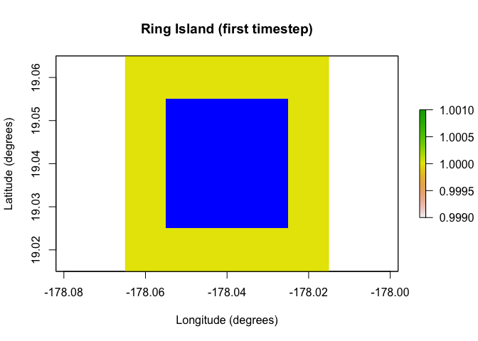
raster::plot(region$temporal_mask_raster()[[10]], main = "Ring Island (last timestep)",
             xlab = "Longitude (degrees)", ylab = "Latitude (degrees)",
             colNA = "blue")
paleopop also includes the PaleoPopModel
class, which sets up the population model structure. Here I show a very
minimalist setup of a model template using this class.
model_template <- PaleoPopModel$new(
  region = region, # makes the simulation spatially explicit
  time_steps = 10, # number of time steps to simulate
  years_per_step = 12, # years per generational time-step
  standard_deviation = 0.1, # SD of growth rate
  growth_rate_max = 0.6, # maximum growth rate
  harvest = F, # are the populations harvested?
  populations = 17, # total occupiable cells over time
  initial_abundance = seq(9000, 0, -1000), # initial pop. sizes
  transition_rate = 1.0, # transition rate between generations
  carrying_capacity = rep(1000, 17), # static carrying capacity
  dispersal = (!diag(nrow = 17, ncol = 17))*0.05, # dispersal rates
  density_dependence = "logistic", # type of density dependence
  dispersal_target_k = 10, # minimum carrying capacity to attract dispersers
  occupancy_threshold = 1, # lower than this # of pops. means extinction
  abundance_threshold = 10, # threshold for Allee effect
  results_selection = c("abundance") # what outputs do you want in results?
)
The paleopop_simulator function accepts a PaleoPopModel
object or a named list as input to simulate populations over paleo time
scales, and the PaleoPopResults class stores the outputs
from the paleo population simulator.
results <- paleopop_simulator(model_template)
results # examine
#> $abundance
#>       [,1] [,2] [,3] [,4] [,5] [,6] [,7] [,8] [,9] [,10]
#>  [1,]   88  150  258  403  606  902 1049  962 1096  1400
#>  [2,]  330  563  733  794  701  781  786  865  964  1104
#>  [3,] 1199 1104  991 1087 1257 1062  998 1016 1025  1055
#>  [4,]  306  465  655  681  954  959  955  934 1008   813
#>  [5,]  101  150  248  369  488  674  826  973 1048  1038
#>  [6,]  336  468  639  687  840  929  972  957 1028   991
#>  [7,]  575  634  888  929  970  907  912 1022 1058   905
#>  [8,] 1123 1086 1140 1215 1140  836  955  934  938   826
#>  [9,]  961  834  908  947 1045  980  964  958 1070   904
#> [10,]    0    0    0    0    0    0    0    0    0     0
#> [11,]    0    0    0    0    0    0    0    0    0     0
#> [12,]    0    0    0    0    0    0    0    0    0     0
#> [13,]  497  666  912 1033  997  972 1023  924  923   929
#> [14,]   64   92  180  258  450  552  761 1039  990  1067
#> [15,]  595  720  881  779 1016  984  933  973 1156  1091
#> [16,]  452  742  850  931  950 1050 1017 1093 1007  1046
#> [17,] 1182 1017 1151 1119  904  689  854  904  890   958
raster::plot(region$raster_from_values(results$abundance[,10]),
             main = "Final abundance", xlab = "Longitude (degrees)",
             ylab = "Latitude (degrees)", colNA = "blue")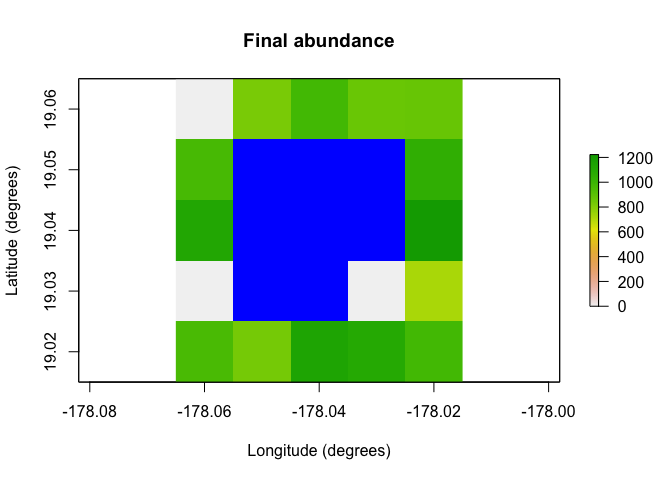
A practical example of how to use paleopop, with more
complex parameterization, can be found in the vignette.
You may cite paleopop in publications using our software
paper in Global Ecology and Biogeography:
Pilowsky, J. A., Haythorne, S., Brown, S. C., Krapp, M., Armstrong, E., Brook, B. W., Rahbek, C., & Fordham, D. A. (2022). Range and extinction dynamics of the steppe bison in Siberia: A pattern‐oriented modelling approach. Global Ecology and Biogeography, 31(12), 2483-2497.