![]()
Tools for Handling Extraction of Features from Time series (theft)
You can install the stable version of theft from
CRAN:
install.packages("theft")You can install the development version of theft from
GitHub using the following:
devtools::install_github("hendersontrent/theft")Please also check out our paper “Feature-Based
Time-Series Analysis in R using the Theft Ecosystem” which discusses
the motivation and theoretical underpinnings of theft and
walks through all of its functionality using the Bonn EEG dataset —
a well-studied neuroscience dataset.
theft is a software package for R that facilitates
user-friendly access to a consistent interface for the extraction of
time-series features. The package provides a single point of access to
\(\approx 6000\) time-series features
from a range of existing R and Python packages as well as enabling users
to calculate their own features. The packages which theft
‘steals’ features from currently are:
Rcatch22 for the native implementation on CRAN)As of v0.6.1, users can also calculate their own
individual features or sets of features too! In addition, two basic
feature sets "quantiles" (a set of 101 quantiles) and
"moments" (the first four moments of the distribution:
mean, variance, skewness, and kurtosis) are also available for users
seeking to compute simple baselines against which to compare the more
sophisticated feature sets (see this recent paper for more
discussion on this idea).
Note that Kats, tsfresh,
TSFEL, and pyhctsa are Python packages.
theft has built-in functionality for helping you install
these libraries—all you need to do is install Python on your machine
(preferably Python >=3.10). If you wish to access the Python feature
sets, please run ?install_python_pkgs in R after
downloading theft or consult the vignette in the package
for more information. For a comprehensive comparison of these six
feature sets across a range of domains (including computation speed,
within-set feature composition, and between-set feature correlations),
please refer to the paper An Empirical
Evaluation of Time-Series Feature Sets.
The companion package theftdlc
(‘theft downloadable content’—just like you get DLCs
and expansions for video games) contains an extensive suite of
functions for analysing, interpreting, and visualising time-series
features calculated from theft. Collectively, these
packages are referred to as the ‘theft ecosystem’.
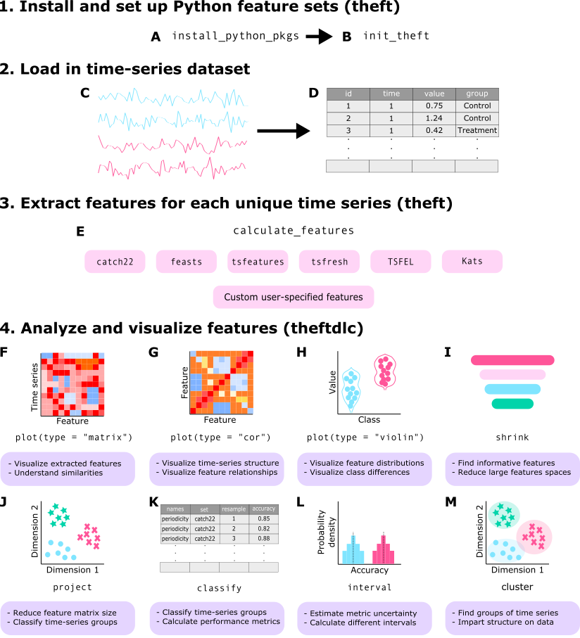
A high-level overview of how the theft ecosystem for R
is typically accessed by users is shown below. Note that prior to
v0.6.1 of, many of the theftdlc functions were
contained in theft but under other names. To ensure the
theft ecosystem is as user-friendly as possible and can
scale to meet future demands, theft has been refactored to
just perform feature extraction, while theftdlc handles all
the processing, analysis, and visualisation of the extracted
features.
Many more functions and options for customisation are available within the packages and users are encouraged to explore the vignettes and helper files for more information.
theft and theftdlc combine to create an
intuitive and efficient workflow consistent with the broader tidyverts collection of
packages for tidy time-series analysis. Here is a single code chunk that
calculates features for a tsibble (tidy
temporal data frame) of some simulated time series processes, including
Gaussian noise, AR(1), ARMA(1,1), MA(1), noisy sinusoid, and a random
walk. simData comes with theft. We’ll just use
the catch22
feature set and a custom set of mean and standard deviation for now.
Using tidy principles and pipes, we can, in the same code chunk, feed
the calculated features straight into theftdlc’s
project function to project the 24-dimensional feature
space into an interpretable two-dimensional space using principal
components analysis:
library(dplyr)
library(theft)
library(theftdlc)

calculate_features(data = theft::simData,
                   feature_set = "catch22",
                   features = list("mean" = mean, "sd" = sd)) %>%
  project(norm_method = "RobustSigmoid",
          unit_int = TRUE,
          low_dim_method = "PCA") %>%
  plot()
In that example, calculate_features comes from
theft, while project and the plot
generic come from theftdlc.
Similarly, we can perform time-series classification using a similar
workflow to compare the performance of catch22 against our
custom set of the first two moments of the distribution:
calculate_features(data = theft::simData,
                   feature_set = "catch22",
                   features = list("mean" = mean, "sd" = sd)) %>%
  classify(by_set = TRUE,
           n_resamples = 10,
           use_null = TRUE) %>%
  compare_features(by_set = TRUE,
                   hypothesis = "pairwise") %>%
  head()
hypothesis feature_set_a feature_set_b metric set_a_mean
1 All features != catch22 All features catch22 accuracy 0.8022222
2 All features != User All features User accuracy 0.8022222
3 catch22 != User catch22 User accuracy 0.7400000
set_b_mean t_statistic p.value
1 0.7400000 2.35154855 0.04319536
2 0.8044444 -0.03932757 0.96948780
3 0.8044444 -1.23794041 0.24705786In this example, classify and
compare_features come from theftdlc.
We can also easily see how each set performs relative to an empirical null distribution (i.e., how much better does each set do than we would expect due to chance?):
calculate_features(data = theft::simData,
                   feature_set = "catch22",
                   features = list("mean" = mean, "sd" = sd)) %>%
  classify(by_set = TRUE,
           n_resamples = 10,
           use_null = TRUE) %>%
  compare_features(by_set = TRUE,
                   hypothesis = "null") %>%
  head()
hypothesis feature_set metric set_mean null_mean
1 All features != own null All features accuracy 0.8022222 0.1355556
2 User != own null User accuracy 0.8044444 0.1511111
3 catch22 != own null catch22 accuracy 0.7400000 0.1222222
t_statistic p.value
1 6.826807 3.835233e-05
2 5.882092 1.171092e-04
3 6.879652 3.614676e-05Please see the vignette for more information and the full functionality of both packages.
If you use theft or theftdlc in your own
work, please cite both the paper:
T. Henderson and Ben D. Fulcher. “Feature-Based Time-Series Analysis in R using the Theft Ecosystem”, The R Journal, 2025.
BibTeX version:
@article{RJ-2025-023,
  author = {Henderson, Trent and Fulcher, Ben D.},
  title = {Feature-Based Time-Series Analysis in R using the Theft Ecosystem},
  journal = {The R Journal},
  year = {2025},
  note = {https://doi.org/10.32614/RJ-2025-023},
  doi = {10.32614/RJ-2025-023},
  volume = {17},
  issue = {3},
  issn = {2073-4859},
  pages = {43-68}
}
and the software:
To cite package 'theft' in publications use:

  Henderson T (2025). _theft: Tools for Handling Extraction of Features
  from Time Series_. R package version 0.8.3,
  <https://hendersontrent.github.io/theft/>.

A BibTeX entry for LaTeX users is

  @Manual{,
    title = {theft: Tools for Handling Extraction of Features from Time Series},
    author = {Trent Henderson},
    year = {2025},
    note = {R package version 0.8.3},
    url = {https://hendersontrent.github.io/theft/},
  }

To cite package 'theftdlc' in publications use:

  Henderson T (2025). _theftdlc: Analyse and Interpret Time Series
  Features_. R package version 0.2.1,
  <https://hendersontrent.github.io/theftdlc/>.

A BibTeX entry for LaTeX users is

  @Manual{,
    title = {theftdlc: Analyse and Interpret Time Series Features},
    author = {Trent Henderson},
    year = {2025},
    note = {R package version 0.2.1},
    url = {https://hendersontrent.github.io/theftdlc/},
}Big thanks to Joshua
Moore for his assistance in solving issues with the Python side of
things and for developing pyhctsa.