| Title: | NFL Logo Plots in 'ggplot2' and 'gt' |
| Version: | 1.6.0 |
| Description: | A set of functions to visualize National Football League analysis in 'ggplot2' plots and 'gt' tables. |
| License: | MIT + file LICENSE |
| URL: | https://nflplotr.nflverse.com, https://github.com/nflverse/nflplotR |
| BugReports: | https://github.com/nflverse/nflplotR/issues |
| Depends: | R (≥ 4.1.0) |
| Imports: | cachem (≥ 1.0.0), cli (≥ 3.0.0), data.table (≥ 1.14.0), ggpath (≥ 1.1.0), ggplot2 (≥ 4.0.0), grid, gt (≥ 0.8.0), lifecycle, magick (≥ 2.7.3), memoise (≥ 2.0.0), nflreadr (≥ 1.5.0), rlang (≥ 1.0.0), S7 (≥ 0.2.0), scales (≥ 1.1.0) |
| Suggests: | base64enc (≥ 0.1-3), colorspace (≥ 2.0), covr, knitr, rmarkdown, rstudioapi (≥ 0.13), rsvg (≥ 2.0), testthat (≥ 3.0.0), vdiffr (≥ 1.0.2), webshot2 (≥ 0.1.1) |
| Config/Needs/website: | mrcaseb/ggpath |
| Config/testthat/edition: | 3 |
| Encoding: | UTF-8 |
| RoxygenNote: | 7.3.3 |
| NeedsCompilation: | no |
| Packaged: | 2025-11-14 15:53:53 UTC; S.Carl |
| Author: | Sebastian Carl [aut, cre] |
| Maintainer: | Sebastian Carl <mrcaseb@gmail.com> |
| Repository: | CRAN |
| Date/Publication: | 2025-11-14 20:30:02 UTC |
nflplotR: NFL Logo Plots in 'ggplot2' and 'gt'
Description
![]()
A set of functions to visualize National Football League analysis in 'ggplot2' plots and 'gt' tables.
Usage
GeomNFLheads

GeomNFLlogo

GeomNFLwordmark
Format
An object of class GeomNFLheads (inherits from Geom, ggproto, gg) of length 5.
An object of class GeomNFLlogo (inherits from Geom, ggproto, gg) of length 5.
An object of class GeomNFLwordmark (inherits from Geom, ggproto, gg) of length 5.
Author(s)
Maintainer: Sebastian Carl mrcaseb@gmail.com
See Also
Useful links:
Report bugs at https://github.com/nflverse/nflplotR/issues
Clear nflplotR Cache
Description
This function clears the memoised cache of all functions memoised by nflplotR.
Usage
.nflplotR_clear_cache()
Value
Invisibly NULL
Examples
.nflplotR_clear_cache()
Theme Elements for Image Grobs
Description
In conjunction with the ggplot2::theme system, the following element_
functions enable images in non-data components of the plot, e.g. axis text.
-
element_nfl_logo(): draws NFL team logos instead of their abbreviations. -
element_nfl_wordmark(): draws NFL team wordmarks instead of their abbreviations. -
element_nfl_headshot(): draws NFL player headshots instead of their GSIS IDs. -
ggpath::element_path(): draws images from valid image URLs instead of the URL.
Usage
element_nfl_logo(
  alpha = 1L,
  colour = NA_character_,
  hjust = 0.5,
  vjust = 0.5,
  color = NULL,
  angle = 0,
  size = grid::unit(0.5, "cm")
)

element_nfl_wordmark(
  alpha = 1L,
  colour = NA_character_,
  hjust = 0.5,
  vjust = 0.5,
  color = NULL,
  angle = 0,
  size = grid::unit(0.5, "cm")
)

element_nfl_headshot(
  alpha = 1L,
  colour = NA_character_,
  hjust = 0.5,
  vjust = 0.5,
  color = NULL,
  angle = 0,
  size = grid::unit(0.5, "cm")
)
Arguments
alpha |
The alpha channel, i.e. transparency level, as a numerical value
between 0 and 1. |
colour, color |
The image will be colorized with this color. Defaults to
|
hjust |
A numeric vector specifying horizontal justification.
If specified, overrides the |
vjust |
A numeric vector specifying vertical justification.
If specified, overrides the |
angle |
The angle of the element as a numerical value between 0° and 360°. |
size |
The output grob size as a grid::unit. If given a numeric,
|
Details
The elements translate NFL team abbreviations or NFL player GSIS IDs into logo images or player headshots, respectively.
Value
An S7 object of class element.
See Also
geom_nfl_logos(), geom_nfl_headshots(), geom_nfl_wordmarks(),
and geom_from_path() for more information on valid team abbreviations,
player IDs, and other parameters.
The examples on https://nflplotr.nflverse.com/articles/nflplotR.html
Examples
library(nflplotR)
library(ggplot2)

team_abbr <- valid_team_names()
# remove conference logos from this example
team_abbr <- team_abbr[!team_abbr %in% c("AFC", "NFC", "NFL")]

df <- data.frame(
  random_value = runif(length(team_abbr), 0, 1),
  teams = team_abbr
)

# use logos for x-axis
ggplot(df, aes(x = teams, y = random_value)) +
  geom_col(aes(color = teams, fill = teams), width = 0.5) +
  scale_color_nfl(type = "secondary") +
  scale_fill_nfl(alpha = 0.4) +
  theme_minimal() +
  theme(axis.text.x.bottom = element_nfl_logo())

# use logos for y-axis
ggplot(df, aes(y = teams, x = random_value)) +
  geom_col(aes(color = teams, fill = teams), width = 0.5) +
  scale_color_nfl(type = "secondary") +
  scale_fill_nfl(alpha = 0.4) +
  theme_minimal() +
  theme(axis.text.y.left = element_nfl_logo())

#############################################################################
# Headshot Examples
#############################################################################
library(nflplotR)
library(ggplot2)

# Silence an nflreadr message that is irrelevant here
old <- options(nflreadr.cache_warning = FALSE)

dfh <- data.frame(
  random_value = runif(9, 0, 1),
  player_gsis = c("00-0033873",
                  "00-0026498",
                  "00-0035228",
                  "00-0031237",
                  "00-0036355",
                  "00-0019596",
                  "00-0033077",
                  "00-0012345",
                  "00-0031280")
)

# use headshots for x-axis
ggplot(dfh, aes(x = player_gsis, y = random_value)) +
  geom_col(width = 0.5) +
  theme_minimal() +
  theme(axis.text.x.bottom = element_nfl_headshot(size = 1))

# use headshots for y-axis
ggplot(dfh, aes(y = player_gsis, x = random_value)) +
  geom_col(width = 0.5) +
  theme_minimal() +
  theme(axis.text.y.left = element_nfl_headshot(size = 1))

# Restore old options
options(old)

#############################################################################
# Wordmarks and other Images
#############################################################################

library(ggplot2)

dt <- data.table::as.data.table(mtcars)[,
  `:=`(
    team = sample(c("LAC", "BUF", "DAL", "ARI"), nrow(mtcars), TRUE),
    player = sample(
      c("00-0033873", "00-0035228", "00-0036355", "00-0019596"),
      nrow(mtcars),
      TRUE
    )
  )
]

ggplot(dt, aes(x = mpg, y = disp)) +
  geom_point() +
  facet_wrap(vars(team)) +
  labs(
    title = tools::toTitleCase("These are random teams and data"),
    subtitle = "I just want to show how the nflplotR theme elements work",
    caption = "https://github.com/nflverse/nflseedR/raw/master/man/figures/caption.png"
  ) +
  theme_minimal() +
  theme(
    plot.title.position = "plot",
    plot.title = element_text(face = "bold"),
    axis.title = element_blank(),
    # make wordmarks of team abbreviations
    strip.text = element_nfl_wordmark(size = 1),
    # load image from url in caption
    plot.caption = element_path(hjust = 1, size = 0.4)
  )
ggplot2 Layer for Visualizing Images from URLs or Local Paths
Description
This geom is used to plot images instead of points in a ggplot. It requires x, y aesthetics as well as a path. It has been outsourced to ggpath and is re-exported in nflplotR for compatibility reasons.
Usage
geom_from_path(...)
Arguments
... |
Arguments passed on to
|
Details
This function has been outsourced to the ggpath package.
See ggpath::geom_from_path for details.
Value
A ggplot2 layer (ggplot2::layer()) that can be added to a plot
created with ggplot2::ggplot().
Aesthetics
geom_from_path() understands the following aesthetics (required aesthetics have no default value):
xThe x-coordinate. Required.
yThe y-coordinate. Required.
patha file path, url, raster object or bitmap array. See
magick::image_read()for further information. Required.alpha = NULLThe alpha channel, i.e. transparency level, as a numerical value between 0 and 1.
colour = NULLThe image will be colorized with this colour. Use the special character
"b/w"to set it to black and white. For more information on valid colour names in ggplot2 see https://ggplot2.tidyverse.org/articles/ggplot2-specs.html?q=colour#colour-and-fillangle = 0The angle of the image as a numerical value between 0° and 360°.
hjust = 0.5The horizontal adjustment relative to the given x coordinate. Must be a numerical value between 0 and 1.
vjust = 0.5The vertical adjustment relative to the given y coordinate. Must be a numerical value between 0 and 1.
width = 1.0The desired width of the image in
npc(Normalised Parent Coordinates). The default value is set to 1.0 which is big but it is necessary because all used values are computed relative to the default. A typical size iswidth = 0.1(see below examples).height = 1.0The desired height of the image in
npc(Normalised Parent Coordinates). The default value is set to 1.0 which is big but it is necessary because all used values are computed relative to the default. A typical size isheight = 0.1(see below examples).
Examples
# example code


library(ggplot2)
library(nflplotR)

# create x-y-coordinates of a pentagon and add nflverse logo urls
df <- data.frame(
  a = c(sin(2 * pi * (0:4) / 5), 0),
  b = c(cos(2 * pi * (0:4) / 5), 0),
  url = c(
    "https://github.com/nflverse/nflfastR/raw/master/man/figures/logo.png",
    "https://github.com/nflverse/nflseedR/raw/master/man/figures/logo.png",
    "https://github.com/nflverse/nfl4th/raw/master/man/figures/logo.png",
    "https://github.com/nflverse/nflreadr/raw/main/data-raw/logo.svg",
    "https://github.com/nflverse/nflplotR/raw/main/man/figures/logo.png",
    "https://github.com/nflverse/nflverse/raw/main/man/figures/logo.png"
  )
)

# plot images directly from url
ggplot(df, aes(x = a, y = b)) +
  geom_from_path(aes(path = url), width = 0.15) +
  coord_cartesian(xlim = c(-2, 2), ylim = c(-1.3, 1.5)) +
  theme_void()

# plot images directly from url and apply transparency
ggplot(df, aes(x = a, y = b)) +
  geom_from_path(aes(path = url), width = 0.15, alpha = 0.5) +
  coord_cartesian(xlim = c(-2, 2), ylim = c(-1.3, 1.5)) +
  theme_void()

# It is also possible and recommended to use the underlying Geom inside a
# ggplot2 annotation
ggplot() +
  annotate(
    ggpath::GeomFromPath,
    x = 0,
    y = 0,
    path = "https://github.com/nflverse/nflplotR/raw/main/man/figures/logo.png",
    width = 0.4
  ) +
  theme_minimal()
ggplot2 Layer for Horizontal and Vertical Reference Lines
Description
These geoms can be used to draw horizontal or vertical reference
lines in a ggplot. They use the data in the aesthetics x0 and y0
to compute their median or mean and draw them as a line.
Usage
geom_median_lines(...)

geom_mean_lines(...)
Arguments
... |
Arguments passed on to
|
Details
These functions have been outsourced to the ggpath package.
See ggpath::geom_median_lines and ggpath::geom_mean_lines for details.
Value
A ggplot2 layer (ggplot2::layer()) that can be added to a plot
created with ggplot2::ggplot().
Aesthetics
geom_median_lines() and geom_mean_lines() understand the following
aesthetics (at least one of the x0 or y0 aesthetics is required):
x0The variable for which to compute the median/mean that is drawn as vertical line.
y0The variable for which to compute the median/mean that is drawn as horizontal line.
alpha = NAThe alpha channel, i.e. transparency level, as a numerical value between 0 and 1.
color = "red"The color of the drawn lines.
linetype = 2The linetype of the drawn lines.
linewidth = 0.5The width of the drawn lines.
See Also
The underlying ggplot2 geoms ggplot2::geom_hline and ggplot2::geom_vline
Examples
library(ggplot2)

# inherit top level aesthetics
ggplot(mtcars, aes(x = disp, y = mpg, y0 = mpg, x0 = disp)) +
  geom_point() +
  geom_median_lines() +
  geom_mean_lines(color = "blue") +
  theme_minimal()

# draw horizontal line only
ggplot(mtcars, aes(x = disp, y = mpg, y0 = mpg)) +
  geom_point() +
  geom_median_lines() +
  geom_mean_lines(color = "blue") +
  theme_minimal()

# draw vertical line only
ggplot(mtcars, aes(x = disp, y = mpg, x0 = disp)) +
  geom_point() +
  geom_median_lines() +
  geom_mean_lines(color = "blue") +
  theme_minimal()

# choose your own value
ggplot(mtcars, aes(x = disp, y = mpg)) +
  geom_point() +
  geom_median_lines(x0 = 400, y0 = 15) +
  geom_mean_lines(x0 = 150, y0 = 30, color = "blue") +
  theme_minimal()
ggplot2 Layer for Visualizing NFL Player Headshots
Description
This geom is used to plot NFL player headshots instead of points in a ggplot. It requires x, y aesthetics as well as a valid NFL player gsis id.
Usage
geom_nfl_headshots(
  mapping = NULL,
  data = NULL,
  stat = "identity",
  position = "identity",
  ...,
  na.rm = FALSE,
  show.legend = FALSE,
  inherit.aes = TRUE
)
Arguments
mapping |
Set of aesthetic mappings created by |
data |
The data to be displayed in this layer. There are three options: If A A |
stat |
The statistical transformation to use on the data for this layer.
When using a
|
position |
A position adjustment to use on the data for this layer. This
can be used in various ways, including to prevent overplotting and
improving the display. The
|
... |
Other arguments passed on to |
na.rm |
If |
show.legend |
logical. Should this layer be included in the legends?
|
inherit.aes |
If |
Value
A ggplot2 layer (ggplot2::layer()) that can be added to a plot
created with ggplot2::ggplot().
Aesthetics
geom_nfl_headshots() understands the following aesthetics (required aesthetics have no default value):
xThe x-coordinate. Required.
yThe y-coordinate. Required.
player_gsisThe players' NFL gsis id. Required.
alpha = NULLThe alpha channel, i.e. transparency level, as a numerical value between 0 and 1.
colour = NULLThe image will be colorized with this colour. Use the special character
"b/w"to set it to black and white. For more information on valid colour names in ggplot2 see https://ggplot2.tidyverse.org/articles/ggplot2-specs.html?q=colour#colour-and-fillangle = 0The angle of the image as a numerical value between 0° and 360°.
hjust = 0.5The horizontal adjustment relative to the given x coordinate. Must be a numerical value between 0 and 1.
vjust = 0.5The vertical adjustment relative to the given y coordinate. Must be a numerical value between 0 and 1.
width = 1.0The desired width of the image in
npc(Normalised Parent Coordinates). The default value is set to 1.0 which is big but it is necessary because all used values are computed relative to the default. A typical size iswidth = 0.075(see below examples).height = 1.0The desired height of the image in
npc(Normalised Parent Coordinates). The default value is set to 1.0 which is big but it is necessary because all used values are computed relative to the default. A typical size isheight = 0.1(see below examples).
Examples
library(nflplotR)
library(ggplot2)
# Silence an nflreadr message that is irrelevant here
old <- options(nflreadr.cache_warning = FALSE)

df <- data.frame(
  a = rep(1:3, 3),
  b = sort(rep(1:3, 3), decreasing = TRUE),
  player_gsis = c("00-0033873",
                  "00-0026498",
                  "00-0035228",
                  "00-0031237",
                  "00-0036355",
                  "00-0019596",
                  "00-0033077",
                  "00-0012345",
                  "00-0031280"),
  player_name = c("P.Mahomes",
                  "M.Stafford",
                  "K.Murray",
                  "T.Bridgewater",
                  "J.Herbert",
                  "T.Brady",
                  "D.Prescott",
                  "Non.Match",
                  "D.Carr")
)

# set a custom fill colour for one player
df$colour <- ifelse(df$a == 2 & df$b == 2, NA, "b/w")

# scatterplot of the headshots
ggplot(df, aes(x = a, y = b)) +
  geom_nfl_headshots(aes(player_gsis = player_gsis), height = 0.2) +
  geom_label(aes(label = player_name), nudge_y = -0.35, alpha = 0.5) +
  coord_cartesian(xlim = c(0.75, 3.25), ylim = c(0.7, 3.25)) +
  theme_void()

# apply alpha as constant
ggplot(df, aes(x = a, y = b)) +
  geom_nfl_headshots(aes(player_gsis = player_gsis), height = 0.2, alpha = 0.5) +
  geom_label(aes(label = player_name), nudge_y = -0.35, alpha = 0.5) +
  coord_cartesian(xlim = c(0.75, 3.25), ylim = c(0.7, 3.25)) +
  theme_void()

# apply colour as an aesthetic
ggplot(df, aes(x = a, y = b)) +
  geom_nfl_headshots(aes(player_gsis = player_gsis, colour = colour), height = 0.2) +
  geom_label(aes(label = player_name), nudge_y = -0.35, alpha = 0.5) +
  coord_cartesian(xlim = c(0.75, 3.25), ylim = c(0.7, 3.25)) +
  scale_colour_identity() +
  theme_void()

# Restore old options
options(old)
ggplot2 Layer for Visualizing NFL Team Logos
Description
This geom is used to plot NFL team and conference logos instead
of points in a ggplot. It requires x, y aesthetics as well as a valid NFL
team abbreviation. The latter can be checked with valid_team_names().
Usage
geom_nfl_logos(
  mapping = NULL,
  data = NULL,
  stat = "identity",
  position = "identity",
  ...,
  na.rm = FALSE,
  show.legend = FALSE,
  inherit.aes = TRUE
)
Arguments
mapping |
Set of aesthetic mappings created by |
data |
The data to be displayed in this layer. There are three options: If A A |
stat |
The statistical transformation to use on the data for this layer.
When using a
|
position |
A position adjustment to use on the data for this layer. This
can be used in various ways, including to prevent overplotting and
improving the display. The
|
... |
Other arguments passed on to |
na.rm |
If |
show.legend |
logical. Should this layer be included in the legends?
|
inherit.aes |
If |
Value
A ggplot2 layer (ggplot2::layer()) that can be added to a plot
created with ggplot2::ggplot().
Aesthetics
geom_nfl_logos() understands the following aesthetics (required aesthetics have no default value):
xThe x-coordinate. Required.
yThe y-coordinate. Required.
team_abbrThe team abbreviation. Should be one of
valid_team_names(). The function tries to clean team names internally by callingnflreadr::clean_team_abbrs(). Note:"NFL","AFC","NFC"are valid abbreviations! Required.alpha = NULLThe alpha channel, i.e. transparency level, as a numerical value between 0 and 1.
colour = NULLThe image will be colorized with this colour. Use the special character
"b/w"to set it to black and white. For more information on valid colour names in ggplot2 see https://ggplot2.tidyverse.org/articles/ggplot2-specs.html?q=colour#colour-and-fillangle = 0The angle of the image as a numerical value between 0° and 360°.
hjust = 0.5The horizontal adjustment relative to the given x coordinate. Must be a numerical value between 0 and 1.
vjust = 0.5The vertical adjustment relative to the given y coordinate. Must be a numerical value between 0 and 1.
width = 1.0The desired width of the image in
npc(Normalised Parent Coordinates). The default value is set to 1.0 which is big but it is necessary because all used values are computed relative to the default. A typical size iswidth = 0.075(see below examples).height = 1.0The desired height of the image in
npc(Normalised Parent Coordinates). The default value is set to 1.0 which is big but it is necessary because all used values are computed relative to the default. A typical size isheight = 0.1(see below examples).
Examples
library(nflplotR)
library(ggplot2)

team_abbr <- valid_team_names()
# remove conference logos from this example
team_abbr <- team_abbr[!team_abbr %in% c("AFC", "NFC", "NFL")]

df <- data.frame(
  a = rep(1:8, 4),
  b = sort(rep(1:4, 8), decreasing = TRUE),
  teams = team_abbr
)

# keep alpha == 1 for all teams including an "A"
matches <- grepl("A", team_abbr)
df$alpha <- ifelse(matches, 1, 0.2)
# also set a custom fill colour for the non "A" teams
df$colour <- ifelse(matches, NA, "gray")

# scatterplot of all logos
ggplot(df, aes(x = a, y = b)) +
  geom_nfl_logos(aes(team_abbr = teams), width = 0.075) +
  geom_label(aes(label = teams), nudge_y = -0.35, alpha = 0.5) +
  expand_limits(y = c(0.9, 4.1)) +
  theme_void()

# apply alpha via an aesthetic from inside the dataset `df`
# please note that you have to add scale_alpha_identity() to use the alpha
# values in your dataset!
ggplot(df, aes(x = a, y = b)) +
  geom_nfl_logos(aes(team_abbr = teams, alpha = alpha), width = 0.075) +
  geom_label(aes(label = teams), nudge_y = -0.35, alpha = 0.5) +
  expand_limits(y = c(0.9, 4.1)) +
  scale_alpha_identity() +
  theme_void()

# apply alpha and colour via an aesthetic from inside the dataset `df`
# please note that you have to add scale_alpha_identity() as well as
# scale_color_identity() to use the alpha and colour values in your dataset!
ggplot(df, aes(x = a, y = b)) +
  geom_nfl_logos(aes(team_abbr = teams, alpha = alpha, colour = colour), width = 0.075) +
  geom_label(aes(label = teams), nudge_y = -0.35, alpha = 0.5) +
  expand_limits(y = c(0.9, 4.1)) +
  scale_alpha_identity() +
  scale_color_identity() +
  theme_void()

# apply alpha as constant for all logos
ggplot(df, aes(x = a, y = b)) +
  geom_nfl_logos(aes(team_abbr = teams), width = 0.075, alpha = 0.6) +
  geom_label(aes(label = teams), nudge_y = -0.35, alpha = 0.5) +
  expand_limits(y = c(0.9, 4.1)) +
  theme_void()

# it's also possible to plot NFL and conference logos
dat <- data.frame(a = c(1.5, 1:2), b = c(1, 0, 0), teams = c("NFL", "AFC", "NFC"))
ggplot(dat, aes(x = a, y = b)) +
  geom_nfl_logos(aes(team_abbr = teams), width = 0.25) +
  coord_cartesian(xlim = c(0.5,2.5), ylim = c(-0.75, 1.75)) +
  theme_void()
ggplot2 Layer for Visualizing NFL Team Wordmarks
Description
This geom is used to plot NFL team wordmarks instead
of points in a ggplot. It requires x, y aesthetics as well as a valid NFL
team abbreviation. The latter can be checked with valid_team_names().
Usage
geom_nfl_wordmarks(
  mapping = NULL,
  data = NULL,
  stat = "identity",
  position = "identity",
  ...,
  na.rm = FALSE,
  show.legend = FALSE,
  inherit.aes = TRUE
)
Arguments
mapping |
Set of aesthetic mappings created by |
data |
The data to be displayed in this layer. There are three options: If A A |
stat |
The statistical transformation to use on the data for this layer.
When using a
|
position |
A position adjustment to use on the data for this layer. This
can be used in various ways, including to prevent overplotting and
improving the display. The
|
... |
Other arguments passed on to |
na.rm |
If |
show.legend |
logical. Should this layer be included in the legends?
|
inherit.aes |
If |
Value
A ggplot2 layer (ggplot2::layer()) that can be added to a plot
created with ggplot2::ggplot().
Aesthetics
geom_nfl_logos() understands the following aesthetics (required aesthetics have no default value):
xThe x-coordinate. Required.
yThe y-coordinate. Required.
team_abbrThe team abbreviation. Should be one of
valid_team_names(). The function tries to clean team names internally by callingnflreadr::clean_team_abbrs(). Required.alpha = NULLThe alpha channel, i.e. transparency level, as a numerical value between 0 and 1.
colour = NULLThe image will be colorized with this colour. Use the special character
"b/w"to set it to black and white. For more information on valid colour names in ggplot2 see https://ggplot2.tidyverse.org/articles/ggplot2-specs.html?q=colour#colour-and-fillangle = 0The angle of the image as a numerical value between 0° and 360°.
hjust = 0.5The horizontal adjustment relative to the given x coordinate. Must be a numerical value between 0 and 1.
vjust = 0.5The vertical adjustment relative to the given y coordinate. Must be a numerical value between 0 and 1.
width = 1.0The desired width of the image in
npc(Normalised Parent Coordinates). The default value is set to 1.0 which is big but it is necessary because all used values are computed relative to the default. A typical size iswidth = 0.1(see below examples).height = 1.0The desired height of the image in
npc(Normalised Parent Coordinates). The default value is set to 1.0 which is big but it is necessary because all used values are computed relative to the default. A typical size isheight = 0.1(see below examples).
Examples
library(nflplotR)
library(ggplot2)

team_abbr <- valid_team_names()
# remove conference logos from this example
team_abbr <- team_abbr[!team_abbr %in% c("AFC", "NFC", "NFL")]

df <- data.frame(
  a = rep(1:8, 4),
  b = sort(rep(1:4, 8), decreasing = TRUE),
  teams = team_abbr
)

# keep alpha == 1 for all teams including an "A"
matches <- grepl("A", team_abbr)
df$alpha <- ifelse(matches, 1, 0.2)
# also set a custom fill colour for the non "A" teams
df$colour <- ifelse(matches, NA, "gray")

# scatterplot of all wordmarks
ggplot(df, aes(x = a, y = b)) +
  geom_nfl_wordmarks(aes(team_abbr = teams), width = 0.12) +
  geom_label(aes(label = teams), nudge_y = -0.20, alpha = 0.5) +
  scale_x_continuous(expand = expansion(add = 0.5)) +
  theme_void()

# apply alpha via an aesthetic from inside the dataset `df`
# please note that you have to add scale_alpha_identity() to use the alpha
# values in your dataset!
ggplot(df, aes(x = a, y = b)) +
  geom_nfl_wordmarks(aes(team_abbr = teams, alpha = alpha), width = 0.12) +
  geom_label(aes(label = teams), nudge_y = -0.20, alpha = 0.5) +
  scale_x_continuous(expand = expansion(add = 0.5)) +
  scale_alpha_identity() +
  theme_void()

# apply alpha and colour via an aesthetic from inside the dataset `df`
# please note that you have to add scale_alpha_identity() as well as
# scale_color_identity() to use the alpha and colour values in your dataset!
ggplot(df, aes(x = a, y = b)) +
  geom_nfl_wordmarks(aes(team_abbr = teams, alpha = alpha, colour = colour), width = 0.12) +
  geom_label(aes(label = teams), nudge_y = -0.20, alpha = 0.5) +
  scale_x_continuous(expand = expansion(add = 0.5)) +
  scale_alpha_identity() +
  scale_color_identity() +
  theme_void()

# apply alpha as constant for all logos
ggplot(df, aes(x = a, y = b)) +
  geom_nfl_wordmarks(aes(team_abbr = teams), width = 0.12, alpha = 0.6) +
  geom_label(aes(label = teams), nudge_y = -0.20, alpha = 0.5) +
  scale_x_continuous(expand = expansion(add = 0.5)) +
  theme_void()
Preview ggplot in Specified Dimensions
Description
This function previews a ggplot in its actual dimensions in order to see how it will look when saved. It is also significantly faster than the default preview in RStudio for ggplots created using nflplotR.
Usage
ggpreview(
  plot = ggplot2::last_plot(),
  width = NA,
  height = NA,
  asp = NULL,
  dpi = 300,
  device = "png",
  units = c("in", "cm", "mm", "px"),
  scale = 1,
  limitsize = TRUE,
  bg = NULL,
  ...
)
Arguments
plot |
Plot to save, defaults to last plot displayed. |
width, height |
Plot size in units expressed by the |
asp |
The aspect ratio of the plot calculated as |
dpi |
Plot resolution. Also accepts a string input: "retina" (320), "print" (300), or "screen" (72). Only applies when converting pixel units, as is typical for raster output types. |
device |
Device to use. Can either be a device function
(e.g. png), or one of "eps", "ps", "tex" (pictex),
"pdf", "jpeg", "tiff", "png", "bmp", "svg" or "wmf" (windows only). If
|
units |
One of the following units in which the |
scale |
Multiplicative scaling factor. |
limitsize |
When |
bg |
Background colour. If |
... |
Other arguments passed on to the graphics device function,
as specified by |
Value
No return value, called for side effects.
Examples
library(nflplotR)
library(ggplot2)

team_abbr <- valid_team_names()
# remove conference logos from this example
team_abbr <- team_abbr[!team_abbr %in% c("AFC", "NFC", "NFL")]

df <- data.frame(
  random_value = runif(length(team_abbr), 0, 1),
  teams = team_abbr
)

# use logos for x-axis
# note that the plot is assigned to the object "p"
p <- ggplot(df, aes(x = teams, y = random_value)) +
  geom_col(aes(color = teams, fill = teams), width = 0.5) +
  scale_color_nfl(type = "secondary") +
  scale_fill_nfl(alpha = 0.4) +
  theme_minimal() +
  theme(axis.text.x = element_nfl_logo())

# preview p with defined width and aspect ratio (only available in RStudio)
if (rstudioapi::isAvailable()){
  ggpreview(p, width = 5, asp = 16/9)
}
Render Logos, Wordmarks, and Headshots in 'gt' Table Column Labels
Description
Translate NFL team abbreviations into logos and wordmarks or NFL player gsis IDs to player headshots and render these images in column labels of 'gt' tables.
Usage
gt_nfl_cols_label(
  gt_object,
  columns = gt::everything(),
  ...,
  height = 30,
  type = c("logo", "wordmark", "headshot")
)
Arguments
gt_object |
A table object that is created using the |
columns |
The columns for which the image translation should be applied.
Argument has no effect if |
... |
Currently not in use |
height |
The absolute height (px) of the image in the table cell. |
type |
One of |
Value
An object of class gt_tbl.
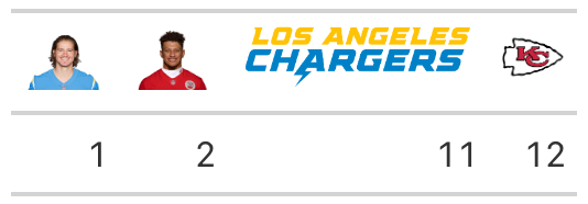
Output of below example
See Also
The article that describes how nflplotR works with the 'gt' package https://nflplotr.nflverse.com/articles/gt.html
The logo and wordmark rendering functions gt_nfl_logos() and
gt_nfl_wordmarks().
The player headshot rendering function gt_nfl_headshots().
Examples
library(gt)
label_df <- data.frame(
  "00-0036355" = 1,
  "00-0033873" = 2,
  "LAC" = 11,
  "KC" = 12,
  check.names = FALSE
)

# create gt table and translate player IDs and team abbreviations
# into headshots, logos, and wordmarks
table <- gt::gt(label_df) |>
  nflplotR::gt_nfl_cols_label(
    columns = gt::starts_with("00"),
    type = "headshot"
  ) |>
  nflplotR::gt_nfl_cols_label("LAC", type = "wordmark") |>
  nflplotR::gt_nfl_cols_label("KC", type = "logo")
Render Player Headshots in 'gt' Tables
Description
Translate NFL player gsis IDs to player headshots and render these images in html tables with the 'gt' package.
Usage
gt_nfl_headshots(gt_object, columns, height = 30, locations = NULL)
Arguments
gt_object |
A table object that is created using the |
columns |
The columns for which the image translation should be applied.
Argument has no effect if |
height |
The absolute height (px) of the image in the table cell. |
locations |
If |
Value
An object of class gt_tbl.
Output of below example

See Also
The logo and wordmark rendering functions gt_nfl_logos() and
gt_nfl_wordmarks().
Examples
library(nflplotR)
library(gt)
# Silence an nflreadr message that is irrelevant here
old <- options(nflreadr.cache_warning = FALSE)
df <- data.frame(
  player_gsis = c("00-0033873",
                  "00-0026498",
                  "00-0035228",
                  "00-0031237",
                  "00-0036355",
                  "00-0019596",
                  "00-0033077",
                  "00-0012345",
                  "00-0031280"),
  player_name = c("P.Mahomes",
                  "M.Stafford",
                  "K.Murray",
                  "T.Bridgewater",
                  "J.Herbert",
                  "T.Brady",
                  "D.Prescott",
                  "Non.Match",
                  "D.Carr")
)

# Replace player IDs with headshot images
table <- gt(df) |>
  gt_nfl_headshots("player_gsis")

# Restore old options
options(old)
Render Logos and Wordmarks in 'gt' Tables
Description
Translate NFL team abbreviations into logos and wordmarks and render these images in html tables with the 'gt' package.
Usage
gt_nfl_logos(gt_object, columns, height = 30, locations = NULL)

gt_nfl_wordmarks(gt_object, columns, height = 30, locations = NULL)
Arguments
gt_object |
A table object that is created using the |
columns |
The columns for which the image translation should be applied.
Argument has no effect if |
height |
The absolute height (px) of the image in the table cell. |
locations |
If |
Value
An object of class gt_tbl.
Output of below example
![]()
See Also
The player headshot rendering function gt_nfl_headshots().
The article that describes how nflplotR works with the 'gt' package https://nflplotr.nflverse.com/articles/gt.html
Examples
library(gt)
library(nflplotR)
teams <- valid_team_names()
# remove conference logos from this example
teams <- teams[!teams %in% c("AFC", "NFC", "NFL")]
# create dataframe with all 32 team names
df <- data.frame(
  team_a = head(teams, 16),
  logo_a = head(teams, 16),
  wordmark_a = head(teams, 16),
  team_b = tail(teams, 16),
  logo_b = tail(teams, 16),
  wordmark_b = tail(teams, 16)
)
# create gt table and translate team names to logo/wordmark images
table <- df |>
  gt() |>
  gt_nfl_logos(columns = gt::starts_with("logo")) |>
  gt_nfl_wordmarks(columns = gt::starts_with("wordmark"))
Format Columns of 'gt' Tables as Percentage Bars
Description
Add context to your data by adding a percentile bar to the actual values. The percentile bar is colored with a color scale based on a user supplied color palette and the relative width of the bars will be rendered as tooltip.
Usage
gt_pct_bar(
  gt_tbl,
  col_value,
  col_pct,
  ...,
  rows = gt::everything(),
  hide_col_pct = FALSE,
  value_position = c("inline", "above"),
  value_scale = 1L,
  value_padding_left = "0px",
  value_padding_right = "0px",
  value_colors = c("black", "white"),
  value_style.props = list(),
  fill_palette = "hulk",
  fill_palette.reverse = FALSE,
  fill_na.color = "#808080",
  fill_pct.domain = 0:100,
  fill_border.color = "transparent",
  fill_border.radius = "10px",
  fill_height = "100%",
  fill_style.props = list(),
  background_border.color = "thin solid black",
  background_border.radius = "12px",
  background_fill.color = "#b1b1b1",
  background_fill.width = "100%",
  background_fill.height = "100%",
  background_style.props = list()
)
Arguments
gt_tbl |
A table object that is created using the |
col_value |
Column name of the value to be printed. |
col_pct |
Column name of percentage values controlling the fill width.
If this is not in a 0 - 100 range, use |
... |
These dots are for future extensions and must be empty. |
rows |
Rows to target
In conjunction with |
hide_col_pct |
If |
value_position |
One of the following:
|
value_scale |
A scaling factor: values from column |
value_padding_left |
Left padding of the printed text. |
value_padding_right |
Right padding of the printed text. |
value_colors |
One or more colors of the printed text. If this is a
vector of colors and |
value_style.props |
A named list of the form |
fill_palette |
The colors that values will be mapped to. This can also
be one of |
fill_palette.reverse |
Whether the vector of colors in |
fill_na.color |
Fill color in case of |
fill_pct.domain |
The possible values that colors in |
fill_border.color |
Border color of color filled area. |
fill_border.radius |
Border radius of color filled area. |
fill_height |
The height of the colored fill bar. Should correspond with
|
fill_style.props |
A named list of the form |
background_border.color |
Border color of background. |
background_border.radius |
Border radius of background. |
background_fill.color |
Fill color of background. |
background_fill.width |
Width of background. |
background_fill.height |
The height of the colored background bar.
Should correspond with |
background_style.props |
A named list of the form |
Details
The function allows extensive styling of the bars and text, either by using
some of the default arguments or, if you want full control, by using the
*_style.props lists which give you full control over all style properties.
All styling parameters are interpreted as style properties of a html span tag.
For more information on CSS properties, see
https://www.w3schools.com/cssref/index.php.
Some notes about styling
Since this is meant to be an extension of an already existing 'gt' table,
you'll have to do some styling outside of this function, esp. the horizontal
alignment and direction will be controlled by gt::cols_align (see example).
Make sure to play around with fill_border.radius and
background_border.radius. Results will depend on final column width and
percentiles. Very short percentile bars, i.e. small values in col_pct,
might result in bars crossing the border when combined with a
big border radius.
Text alignment depending on the colored bar isn't as easy as one might think.
Try percent values in value_padding_left or value_padding_right to avoid
overlapping of text values and the outline of the colored bars.
For more information and examples, see the article that describes how nflplotR works with the 'gt' package https://nflplotr.nflverse.com/articles/gt.html.
Value
An object of class gt_tbl.
Output of below example

See Also
The article that describes how nflplotR works with the 'gt' package https://nflplotr.nflverse.com/articles/gt.html
Examples
library(data.table)

# Make a data.table of mtcars and select only disp and hp
data <- data.table::as.data.table(mtcars)[, list(disp, hp)]

# Add the percentile of hp in the distribution of hp values
data[, pct := round(stats::ecdf(hp)(hp) * 100, 1)]

# set seed to keep it reproducible
set.seed(20)

# take random sample (to avoid a big table) and add the percent bars for hp
# using the percentiles in the pct variable
table <- data[sample(.N, 10)] |>
  gt::gt() |>
  nflplotR::gt_pct_bar(
    "hp", "pct",
    hide_col_pct = FALSE,
    value_padding_left = "10px",
  ) |>
  gt::cols_align("left", hp) |>
  gt::cols_width(hp ~ gt::px(250))
Render 'gt' Table to Temporary png File
Description
Saves a gt table to a temporary png image file and uses magick to render
tables in reproducible examples like reprex::reprex() or in package
function examples (see details for further information).
Usage
gt_render_image(gt_tbl, ...)
Arguments
gt_tbl |
An object of class |
... |
Arguments passed on to |
Details
Rendering gt tables in function examples is not trivial because
of the behavior of an underlying dependency: chromote. It keeps a process
running even if the chromote session is closed. Unfortunately, this causes
R CMD Check errors related to open connections after example runs. The only
way to avoid this is setting the environment variable _R_CHECK_CONNECTIONS_LEFT_OPEN_
to "false". How to do that depends on where and how developers check their
package. A good way to prevent an example from being executed because the
environment variable was not set to "false" can be taken from the source
code of this function.
Value
Returns NULL invisibly.
Examples
tbl <- gt::gt_preview(mtcars)
gt_render_image(tbl)
Create Ordered NFL Team Name Factor
Description
Create Ordered NFL Team Name Factor
Usage
nfl_team_factor(teams, ...)
Arguments
teams |
A vector of NFL team abbreviations that should be included in
|
... |
One or more unquoted column names of |
Value
Object of class "factor"
Examples
# unsorted vector including NFL team abbreviations
teams <- c("LAC", "LV", "CLE", "BAL", "DEN", "PIT", "CIN", "KC")

# defaults to sort by division and nick name in ascending order
nfl_team_factor(teams)

# can sort by every column in nflreadr::load_teams()
nfl_team_factor(teams, team_abbr)

# descending order by using base::rev()
nfl_team_factor(teams, rev(team_abbr))

######### HOW TO USE IN PRACTICE #########

library(ggplot2)
# load some sample data from the ggplot2 package
plot_data <- mpg
# add a new column by randomly sampling the above defined teams vector
plot_data$team <- sample(teams, nrow(mpg), replace = TRUE)

# Now we plot the data and facet by team abbreviation. ggplot automatically
# converts the team names to a factor and sorts it alphabetically
ggplot(plot_data, aes(displ, hwy)) +
  geom_point() +
  facet_wrap(~team, ncol = 4) +
  theme_minimal()

# We'll change the order of facets by making another team name column and
# converting it to an ordered factor. Again, this defaults to sort by division
# and nick name in ascending order.
plot_data$ordered_team <- nfl_team_factor(sample(teams, nrow(mpg), replace = TRUE))

# Let's check how the facets are ordered now.
ggplot(plot_data, aes(displ, hwy)) +
  geom_point() +
  facet_wrap(~ordered_team, ncol = 4) +
  theme_minimal()

# The facet order looks weird because the defaults is meant to be used with
# NFL team wordmarks. So let's use the actual wordmarks and look at the result.
ggplot(plot_data, aes(displ, hwy)) +
  geom_point() +
  facet_wrap(~ordered_team, ncol = 4) +
  theme_minimal() +
  theme(strip.text = element_nfl_wordmark())
Create NFL Team Tiers
Description
This function sets up a ggplot to visualize NFL team tiers.
Usage
nfl_team_tiers(
  data,
  title = "NFL Team Tiers, 2021 as of Week 4",
  subtitle = "created with the #nflplotR Tiermaker",
  caption = NULL,
  tier_desc = c(`1` = "Super Bowl", `2` = "Very Good", `3` = "Medium", `4` = "Bad", `5` =
    "What are they doing?", `6` = "", `7` = ""),
  presort = FALSE,
  alpha = 0.8,
  width = 0.075,
  no_line_below_tier = NULL,
  devel = FALSE
)
Arguments
data |
A data frame that has to include the variables |
title |
The title of the plot. If |
subtitle |
The subtitle of the plot. If |
caption |
The caption of the plot. If |
tier_desc |
A named vector consisting of the tier descriptions. The names
must equal the tier numbers from |
presort |
If |
alpha |
The alpha channel of the logos, i.e. transparency level, as a numerical value between 0 and 1. |
width |
The desired width of the logo in |
no_line_below_tier |
Vector of tier numbers. The function won't draw tier separation lines below these tiers. This is intended to be used for tiers that shall be combined (see examples). |
devel |
Determines if logos shall be rendered. If |
Value
A plot object created with ggplot2::ggplot().
Examples
library(ggplot2)
library(data.table)
teams <- nflplotR::valid_team_names()
# remove conference logos from this example
teams <- teams[!teams %in% c("AFC", "NFC", "NFL")]
teams <- sample(teams)

# Build the team tiers data
# This is completely random!
dt <- data.table::data.table(
  tier_no = sample(1:5, length(teams), replace = TRUE),
  team_abbr = teams
)[,tier_rank := sample(1:.N, .N), by = "tier_no"]

# Plot team tiers
nfl_team_tiers(dt)

# Create a combined tier which is useful for tiers with lots of teams that
# should be split up in two or more rows. This is done by setting an empty
# string for the tier 5 description and removing the tier separation line
# below tier number 4.
# This example also shows how to turn off the subtitle and add a caption
nfl_team_tiers(dt,
               subtitle = NULL,
               caption = "This is the caption",
               tier_desc = c("1" = "Super Bowl",
                             "2" = "Very Good",
                             "3" = "Medium",
                             "4" = "A Combined Tier",
                             "5" = ""),
               no_line_below_tier = 4)

# For the development of the tiers, it can be useful to turn off logo image
# rendering as this can take quite a long time. By setting `devel = TRUE`, the
# logo images are replaced by team abbreviations which is much faster
nfl_team_tiers(dt,
               tier_desc = c("1" = "Super Bowl",
                             "2" = "Very Good",
                             "3" = "",
                             "4" = "A Combined Tier",
                             "5" = ""),
               no_line_below_tier = c(2, 4),
               devel = TRUE)
Get a Situation Report on System, nflverse Package Versions and Dependencies
Description
See nflreadr::nflverse_sitrep for details.
Value
Situation report of R and package/dependencies.
Objects exported from other packages
Description
These objects are imported from other packages. Follow the links below to see their documentation.
- ggpath
Scales for NFL Team Colors
Description
These functions map NFL team names to their team colors in color and fill aesthetics
Usage
scale_color_nfl(
  type = c("primary", "secondary"),
  values = NULL,
  ...,
  aesthetics = "colour",
  breaks = ggplot2::waiver(),
  na.value = "grey50",
  guide = NULL,
  alpha = NA
)

scale_colour_nfl(
  type = c("primary", "secondary"),
  values = NULL,
  ...,
  aesthetics = "colour",
  breaks = ggplot2::waiver(),
  na.value = "grey50",
  guide = NULL,
  alpha = NA
)

scale_fill_nfl(
  type = c("primary", "secondary"),
  values = NULL,
  ...,
  aesthetics = "fill",
  breaks = ggplot2::waiver(),
  na.value = "grey50",
  guide = NULL,
  alpha = NA
)
Arguments
type |
One of |
values |
If |
... |
Arguments passed on to
|
aesthetics |
Character string or vector of character strings listing the
name(s) of the aesthetic(s) that this scale works with. This can be useful, for
example, to apply colour settings to the |
breaks |
One of:
|
na.value |
The aesthetic value to use for missing ( |
guide |
A function used to create a guide or its name. If |
alpha |
Factor to modify color transparency via a call to |
Examples
library(nflplotR)
library(ggplot2)

team_abbr <- valid_team_names()
# remove conference logos from this example
team_abbr <- team_abbr[!team_abbr %in% c("AFC", "NFC", "NFL")]

df <- data.frame(
  random_value = runif(length(team_abbr), 0, 1),
  teams = team_abbr
)
ggplot(df, aes(x = teams, y = random_value)) +
  geom_col(aes(color = teams, fill = teams), width = 0.5) +
  scale_color_nfl(type = "secondary") +
  scale_fill_nfl(alpha = 0.4) +
  theme_minimal() +
  theme(axis.text.x = element_text(angle = 45, hjust = 1))
Output Valid NFL Team Abbreviations
Description
Output Valid NFL Team Abbreviations
Usage
valid_team_names(exclude_duplicates = TRUE)
Arguments
exclude_duplicates |
If |
Value
A vector of type "character".
Examples
# List valid team abbreviations excluding duplicates
valid_team_names()

# List valid team abbreviations excluding duplicates
valid_team_names(exclude_duplicates = FALSE)