Type:	Package
Title:	Matrix Functions for Teaching and Learning Linear Algebra and Multivariate Statistics
Version:	1.0.0
Date:	2024-09-27
Maintainer:	Michael Friendly <friendly@yorku.ca>
Description:	A collection of matrix functions for teaching and learning matrix linear algebra as used in multivariate statistical methods. These functions are mainly for tutorial purposes in learning matrix algebra ideas using R. In some cases, functions are provided for concepts available elsewhere in R, but where the function call or name is not obvious. In other cases, functions are provided to show or demonstrate an algorithm. In addition, a collection of functions are provided for drawing vector diagrams in 2D and 3D.
License:	GPL-2 | GPL-3 [expanded from: GPL (≥ 2)]
Language:	en-US
URL:	https://github.com/friendly/matlib, http://friendly.github.io/matlib/
BugReports:	https://github.com/friendly/matlib/issues
LazyData:	TRUE
Suggests:	carData, webshot2, markdown, bookdown, clipr
Imports:	xtable, MASS, rgl, car, methods, dplyr, knitr, rmarkdown, rstudioapi
VignetteBuilder:	knitr
RoxygenNote:	7.3.2
Encoding:	UTF-8
NeedsCompilation:	no
Packaged:	2024-10-02 17:48:09 UTC; friendly
Author:	Michael Friendly [aut, cre], John Fox [aut], Phil Chalmers [aut], Georges Monette [ctb], Gaston Sanchez [ctb]
Repository:	CRAN
Date/Publication:	2024-10-02 18:30:10 UTC

matlib: Matrix Functions for Teaching and Learning Linear Algebra and Multivariate Statistics.

Description

These functions are designed mainly for tutorial purposes in teaching & learning matrix algebra ideas and applications to statistical methods using R.

Details

In some cases, functions are provided for concepts available elsewhere in R, but where the function call or name is not obvious. In other cases, functions are provided to show or demonstrate an algorithm, sometimes providing a verbose argument to print the details of computations.

In addition, a collection of functions are provided for drawing vector diagrams in 2D and 3D.

These are not meant for production uses. Other methods are more efficient for larger problems.

Topics

The functions in this package are grouped under the following topics

• Convenience functions:
  tr, R, J, len, vec, Proj, mpower, vandermode

• Determinants: functions for calculating determinants by cofactor expansion
  minor, cofactor, rowMinors, rowCofactors

• Elementary row operations: functions for solving linear equations "manually" by the steps used in row echelon form and Gaussian elimination
  rowadd, rowmult, rowswap

• Linear equations: functions to illustrate linear equations of the form $A x = b$
  showEqn, plotEqn

• Gaussian elimination: functions for illustrating Gaussian elimination for solving systems of linear equations of the form $A x = b$.
  gaussianElimination, Inverse, inv, echelon, Ginv, LU, cholesky, swp

• Eigenvalues: functions to illustrate the algorithms for calculating eigenvalues and eigenvectors
  eigen, SVD, powerMethod, showEig

• Vector diagrams: functions for drawing vector diagrams in 2D and 3D
  arrows3d, corner, arc, pointOnLine, vectors, vectors3d, regvec3d

Most of these ideas and implementations arose in courses and books by the authors. [Psychology 6140](http://friendly.apps01.yorku.ca/psy6140/) was a starting point. Fox (1984) introduced illustrations of vector geometry.

macOS Installation Note

The functions that draw 3D graphs use the rgl package. On macOS, the rgl package requires that XQuartz be installed. After installing XQuartz, it's necessary either to log out of and back into your macOS account or to reboot your Mac.

References

Fox, J. Linear Statistical Models and Related Methods. John Wiley and Sons, 1984

Fox, J. and Friendly, M. (2016). "Visualizing Simultaneous Linear Equations, Geometric Vectors, and Least-Squares Regression with the matlib Package for R". useR Conference, Stanford, CA, June 27 - June 30, 2016.

Determinant of a Square Matrix

Description

Returns the determinant of a square matrix X, computed either by Gaussian elimination, expansion by cofactors, or as the product of the eigenvalues of the matrix. If the latter, X must be symmetric.

Usage

Det(
  X,
  method = c("elimination", "eigenvalues", "cofactors"),
  verbose = FALSE,
  fractions = FALSE,
  ...
)

Arguments

Value

the determinant of X

Author(s)

John Fox

See Also

det for the base R function

gaussianElimination, Eigen

Other determinants: adjoint(), cofactor(), minor(), rowCofactors(), rowMinors()

Examples

A <- matrix(c(1,2,3,2,5,6,3,6,10), 3, 3) # nonsingular, symmetric
A
Det(A)
Det(A, verbose=TRUE, fractions=TRUE)
B <- matrix(1:9, 3, 3) # a singular matrix
B
Det(B)
C <- matrix(c(1, .5, .5, 1), 2, 2) # square, symmetric, nonsingular
Det(C)
Det(C, method="eigenvalues")
Det(C, method="cofactors")

Eigen Decomposition of a Square Symmetric Matrix

Description

Eigen calculates the eigenvalues and eigenvectors of a square, symmetric matrix using the iterated QR decomposition

Usage

Eigen(X, tol = sqrt(.Machine$double.eps), max.iter = 100, retain.zeroes = TRUE)

Arguments

Value

a list of two elements: values– eigenvalues, vectors– eigenvectors

Author(s)

John Fox and Georges Monette

See Also

eigen

SVD

Examples

C <- matrix(c(1,2,3,2,5,6,3,6,10), 3, 3) # nonsingular, symmetric
C
EC <- Eigen(C) # eigenanalysis of C
EC$vectors %*% diag(EC$values) %*% t(EC$vectors) # check

Create a LaTeX Equation Wrapper

Description

The Eqn function is designed to produce LaTeX expressions of mathematical equations for writing. The output can be copied/pasted into documents or used directly in chunks in .Rmd, .Rnw, or .qmd documents to compile to equations. It wraps the equations generated by its arguments in either a \begin{equation} ...\end{equation} or \begin{align} ...\end{align} LaTeX environment. See also ref for consistent inline referencing of numbered equations.

In a code chunk, use the chunk options results='asis', echo=FALSE to show only the result of compiling the LaTeX expressions.

Eqn_newline() emits a newline (\) in an equation, with an optional increase to the padding following the newline.

Eqn_text() inserts a literal string to be rendered in a text font in an equation.

Eqn_hspace() is used to create (symmetric) equation spaces, most typically around = signs Input to lhs, rhs can be a numeric to increase the size of the space or a character vector to be passed to the LaTeX macro \hspace{}.

Eqn_vspace() inserts vertical space between lines in an equation. Typically used for aligned, multiline equations.

Eqn_size() is used to increase or decrease the size of LaTeX text and equations. Can be applied to a specific string or applied to all subsequent text until overwritten.

ref{} provides inline references to equations in R markdown and Quarto documents. Depending on the output type this function will provide the correct inline wrapper for MathJax or LaTeX equations. This provides more consistent referencing when switching between HTML and PDF outputs as well as documentation types (e.g., .Rmd vs .qmd).

Usage

Eqn(
  ...,
  label = NULL,
  align = FALSE,
  preview = getOption("previewEqn"),
  html_output = knitr::is_html_output(),
  quarto = getOption("quartoEqn"),
  mat_args = list(),
  preview.pdf = FALSE,
  preview.packages = NULL
)

Eqn_newline(space = 0)

Eqn_text(text)

Eqn_hspace(lhs = 5, mid = "", rhs = NULL, times = 1)

Eqn_vspace(space)

Eqn_size(string, size = 0)

ref(
  label,
  parentheses = TRUE,
  html_output = knitr::is_html_output(),
  quarto = getOption("quartoEqn")
)

Arguments

Author(s)

Phil Chalmers

See Also

latexMatrix, matrix2latex, ref

Examples

# character input
Eqn('e=mc^2')

# show only the LaTeX code
Eqn('e=mc^2', preview=FALSE)

# Equation numbers & labels
Eqn('e=mc^2', label = 'eq:einstein')
Eqn("X=U \\lambda V", label='eq:svd')

# html_output and quarto outputs only show code
#   (both auto detected in compiled documents)
Eqn('e=mc^2', label = 'eq:einstein', html_output = TRUE)

# Quarto output
Eqn('e=mc^2', label = 'eq-einstein', quarto = TRUE)

## Not run: 
# The following requires LaTeX compilers to be pre-installed

# View PDF instead of HTML
Eqn('e=mc^2', preview.pdf=TRUE)

# Add extra LaTeX dependencies for PDF build
Eqn('\\bm{e}=mc^2', preview.pdf=TRUE,
    preview.packages=c('amsmath', 'bm'))


## End(Not run)

# Multiple expressions
Eqn("e=mc^2",
    Eqn_newline(),
    "X=U \\lambda V", label='eq:svd')

# expressions that use cat() within their calls
Eqn('SVD = ',
    latexMatrix("u", "n", "k"),
    latexMatrix("\\lambda", "k", "k", diag=TRUE),
    latexMatrix("v", "k", "p", transpose = TRUE),
    label='eq:svd')

# align equations using & operator
Eqn("X &= U \\lambda V", Eqn_newline(),
    "& = ", latexMatrix("u", "n", "k"),
    latexMatrix("\\lambda", "k", "k", diag=TRUE),
    latexMatrix("v", "k", "p", transpose = TRUE),
    align=TRUE)

#  numeric/character matrix example
A <- matrix(c(2, 1, -1,
              -3, -1, 2,
              -2,  1, 2), 3, 3, byrow=TRUE)
b <- matrix(c(8, -11, -3))

# numeric matrix wrapped internally
cbind(A,b) |> Eqn()
cbind(A,b) |> latexMatrix() |> Eqn()

# change numeric matrix brackets globally
cbind(A,b) |> Eqn(mat_args=list(matrix='bmatrix'))

# greater flexibility when using latexMatrix()
cbind(A, b) |> latexMatrix() |> partition(columns=3) |> Eqn()

# with showEqn()
showEqn(A, b, latex=TRUE) |> Eqn()


Eqn_newline()
Eqn_newline('10ex')


Eqn_hspace()
Eqn_hspace(3) # smaller
Eqn_hspace(3, times=2)
Eqn_hspace('1cm')

# symmetric spacing around mid
Eqn_hspace(mid='=')
Eqn_hspace(mid='=', times=2)


Eqn_vspace('1.5ex')
Eqn_vspace('1cm')



# set size globally
Eqn_size(size=3)
Eqn_size() # reset

# locally for defined string
string <- 'e = mc^2'
Eqn_size(string, size=1)



# used inside of Eqn() or manually defined labels in the document
Eqn('e = mc^2', label='eq:einstein')

# use within inline block via `r ref()`
ref('eq:einstein')
ref('eq:einstein', parentheses=FALSE)
ref('eq:einstein', html_output=TRUE)

# With Quarto
Eqn('e = mc^2', label='eq-einstein', quarto=TRUE)
ref('eq:einstein', quarto=TRUE)
ref('eq:einstein', quarto=TRUE, parentheses=FALSE)

Generalized Inverse of a Matrix

Description

Ginv returns an arbitrary generalized inverse of the matrix A, using gaussianElimination.

Usage

Ginv(A, tol = sqrt(.Machine$double.eps), verbose = FALSE, fractions = FALSE)

Arguments

Details

A generalized inverse is a matrix \mathbf{A}^- satisfying \mathbf{A A^- A} = \mathbf{A}.

The purpose of this function is mainly to show how the generalized inverse can be computed using Gaussian elimination.

Value

the generalized inverse of A, expressed as fractions if fractions=TRUE, or rounded

Author(s)

John Fox

See Also

ginv for a more generally usable function

Examples

A <- matrix(c(1,2,3,4,5,6,7,8,10), 3, 3) # a nonsingular matrix
A
Ginv(A, fractions=TRUE)  # a generalized inverse of A = inverse of A
round(Ginv(A) %*% A, 6)  # check

B <- matrix(1:9, 3, 3) # a singular matrix
B
Ginv(B, fractions=TRUE)  # a generalized inverse of B
B %*% Ginv(B) %*% B   # check

Gram-Schmidt Orthogonalization of a Matrix

Description

Carries out simple Gram-Schmidt orthogonalization of a matrix. Treating the columns of the matrix X in the given order, each successive column after the first is made orthogonal to all previous columns by subtracting their projections on the current column.

Usage

GramSchmidt(
  X,
  normalize = TRUE,
  verbose = FALSE,
  tol = sqrt(.Machine$double.eps),
  omit_zero_columns = TRUE
)

Arguments

Value

A matrix of the same size as X, with orthogonal columns (but with 0 columns removed by default)

Author(s)

Phil Chalmers, John Fox

Examples

(xx <- matrix(c( 1:3, 3:1, 1, 0, -2), 3, 3))
crossprod(xx)
(zz <- GramSchmidt(xx, normalize=FALSE))
zapsmall(crossprod(zz))

# normalized
(zz <- GramSchmidt(xx))
zapsmall(crossprod(zz))

# print steps
GramSchmidt(xx, verbose=TRUE)

# A non-invertible matrix;  hence, it is of deficient rank
(xx <- matrix(c( 1:3, 3:1, 1, 0, -1), 3, 3))
R(xx)
crossprod(xx)
# GramSchmidt finds an orthonormal basis
(zz <- GramSchmidt(xx))
zapsmall(crossprod(zz))

Inverse of a Matrix

Description

Uses gaussianElimination to find the inverse of a square, non-singular matrix, X.

Usage

Inverse(X, tol = sqrt(.Machine$double.eps), verbose = FALSE, ...)

Arguments

Details

The method is purely didactic: The identity matrix, I, is appended to X, giving X | I. Applying Gaussian elimination gives I | X^{-1}, and the portion corresponding to X^{-1} is returned.

Value

the inverse of X

Author(s)

John Fox

Examples

  A <- matrix(c(2, 1, -1,
               -3, -1, 2,
               -2,  1, 2), 3, 3, byrow=TRUE)
  Inverse(A)
  Inverse(A, verbose=TRUE, fractions=TRUE)

Create a vector, matrix or array of constants

Description

This function creates a vector, matrix or array of constants, typically used for the unit vector or unit matrix in matrix expressions.

Usage

J(..., constant = 1, dimnames = NULL)

Arguments

Details

The "dimnames" attribute is optional: if present it is a list with one component for each dimension, either NULL or a character vector of the length given by the element of the "dim" attribute for that dimension. The list can be named, and the list names will be used as names for the dimensions.

Examples

J(3)
J(2,3)
J(2,3,2)
J(2,3, constant=2, dimnames=list(letters[1:2], LETTERS[1:3]))

X <- matrix(1:6, nrow=2, ncol=3)
dimnames(X) <- list(sex=c("M", "F"), day=c("Mon", "Wed", "Fri"))
J(2) %*% X      # column sums
X %*% J(3)      # row sums

LU Decomposition

Description

LU computes the LU decomposition of a matrix, A, such that P A = L U, where L is a lower triangle matrix, U is an upper triangle, and P is a permutation matrix.

Usage

LU(A, b, tol = sqrt(.Machine$double.eps), verbose = FALSE, ...)

Arguments

Details

The LU decomposition is used to solve the equation A x = b by calculating L(Ux - d) = 0, where Ld = b. If row exchanges are necessary for A then the permutation matrix P will be required to exchange the rows in A; otherwise, P will be an identity matrix and the LU equation will be simplified to A = L U.

Value

A list of matrix components of the solution, P, L and U. If b is supplied, the vectors d and x are also returned.

Author(s)

Phil Chalmers

Examples

  A <- matrix(c(2, 1, -1,
               -3, -1, 2,
               -2,  1, 2), 3, 3, byrow=TRUE)
  b <- c(8, -11, -3)
  (ret <- LU(A)) # P is an identity; no row swapping
  with(ret, L %*% U) # check that A = L * U
  LU(A, b)
  
  LU(A, b, verbose=TRUE)
  LU(A, b, verbose=TRUE, fractions=TRUE)

  # permutations required in this example
  A <- matrix(c(1,  1, -1,
                2,  2,  4,
                1, -1,  1), 3, 3, byrow=TRUE)
  b <- c(1, 2, 9)
  (ret <- LU(A, b))
  with(ret, P %*% A)
  with(ret, L %*% U)

Moore-Penrose inverse of a matrix

Description

The Moore-Penrose inverse is a generalization of the regular inverse of a square, non-singular, symmetric matrix to other cases (rectangular, singular), yet retain similar properties to a regular inverse.

Usage

MoorePenrose(X, tol = sqrt(.Machine$double.eps))

Arguments

Value

The Moore-Penrose inverse of X

Examples

X <- matrix(rnorm(20), ncol=2)
# introduce a linear dependency in X[,3]
X <- cbind(X, 1.5*X[, 1] - pi*X[, 2])

Y <- MoorePenrose(X)
# demonstrate some properties of the M-P inverse
# X Y X = X
round(X %*% Y %*% X - X, 8)
# Y X Y = Y
round(Y %*% X %*% Y - Y, 8)
# X Y = t(X Y)
round(X %*% Y - t(X %*% Y), 8)
# Y X = t(Y X)
round(Y %*% X - t(Y %*% X), 8)

Projection of Vector y on columns of X

Description

Fitting a linear model, lm(y ~ X), by least squares can be thought of geometrically as the orthogonal projection of y on the column space of X. This function is designed to allow exploration of projections and orthogonality.

Usage

Proj(y, X, list = FALSE)

Arguments

Details

The projection is defined as P y where P = X (X'X)^- X' and X^- is a generalized inverse.

Value

the projection of y on X (if list=FALSE) or a list with elements y and P

Author(s)

Michael Friendly

See Also

Other vector diagrams: arc(), arrows3d(), circle3d(), corner(), plot.regvec3d(), pointOnLine(), regvec3d(), vectors(), vectors3d()

Examples

X <- matrix( c(1, 1, 1, 1, 1, -1, 1, -1), 4,2, byrow=TRUE)
y <- 1:4
Proj(y, X[,1])  # project y on unit vector
Proj(y, X[,2])
Proj(y, X)

# project unit vector on line between two points
y <- c(1,1)
p1 <- c(0,0)
p2 <- c(1,0)
Proj(y, cbind(p1, p2))

# orthogonal complements
y <- 1:4
yp <-Proj(y, X, list=TRUE)
yp$y
P <- yp$P
IP <- diag(4) - P
yc <- c(IP %*% y)
crossprod(yp$y, yc)

# P is idempotent:  P P = P
P %*% P
all.equal(P, P %*% P)

QR Decomposition by Graham-Schmidt Orthonormalization

Description

QR computes the QR decomposition of a matrix, X, that is an orthonormal matrix, Q and an upper triangular matrix, R, such that X = Q R.

Usage

QR(X, tol = sqrt(.Machine$double.eps))

Arguments

Details

The QR decomposition plays an important role in many statistical techniques. In particular it can be used to solve the equation Ax = b for given matrix A and vector b. The function is included here simply to show the algorithm of Gram-Schmidt orthogonalization. The standard qr function is faster and more accurate.

Value

a list of three elements, consisting of an orthonormal matrix Q, an upper triangular matrix R, and the rank of the matrix X

Author(s)

John Fox and Georges Monette

See Also

qr

Examples

A <- matrix(c(1,2,3,4,5,6,7,8,10), 3, 3) # a square nonsingular matrix
res <- QR(A)
res
q <- res$Q
zapsmall( t(q) %*% q)   # check that q' q = I
r <- res$R
q %*% r                 # check that q r = A

# relation to determinant: det(A) = prod(diag(R))
det(A)
prod(diag(r))

B <- matrix(1:9, 3, 3) # a singular matrix
QR(B)

Rank of a Matrix

Description

Returns the rank of a matrix X, using the QR decomposition, QR. Included here as a simple function, because rank does something different and it is not obvious what to use for matrix rank.

Usage

R(X)

Arguments

Value

rank of X

See Also

qr

Examples

M <- outer(1:3, 3:1)
M
R(M)

M <- matrix(1:9, 3, 3)
M
R(M)
# why rank=2?
echelon(M)

set.seed(1234)
M <- matrix(sample(1:9), 3, 3)
M
R(M)

Singular Value Decomposition of a Matrix

Description

Compute the singular-value decomposition of a matrix X either by Jacobi rotations (the default) or from the eigenstructure of X'X using Eigen. Both methods are iterative. The result consists of two orthonormal matrices, U, and V and the vector d of singular values, such that X = U diag(d) V'.

Usage

SVD(
  X,
  method = c("Jacobi", "eigen"),
  tol = sqrt(.Machine$double.eps),
  max.iter = 100
)

Arguments

Details

The default method is more numerically stable, but the eigenstructure method is much simpler. Singular values of zero are not retained in the solution.

Value

a list of three elements: d– singular values, U– left singular vectors, V– right singular vectors

Author(s)

John Fox and Georges Monette

See Also

svd, the standard svd function

Eigen

Examples

C <- matrix(c(1,2,3,2,5,6,3,6,10), 3, 3) # nonsingular, symmetric
C
SVD(C)

# least squares by the SVD
data("workers")
X <- cbind(1, as.matrix(workers[, c("Experience", "Skill")]))
head(X)
y <- workers$Income
head(y)
(svd <- SVD(X))
VdU <- svd$V %*% diag(1/svd$d) %*%t(svd$U)
(b <- VdU %*% y)
coef(lm(Income ~ Experience + Skill, data=workers))

Solve and Display Solutions for Systems of Linear Simultaneous Equations

Description

Solve the equation system Ax = b, given the coefficient matrix A and right-hand side vector b, using link{gaussianElimination}. Display the solutions using showEqn.

Usage

Solve(
  A,
  b = rep(0, nrow(A)),
  vars,
  verbose = FALSE,
  simplify = TRUE,
  fractions = FALSE,
  ...
)

Arguments

Details

This function mimics the base function solve when supplied with two arguments, (A, b), but gives a prettier result, as a set of equations for the solution. The call solve(A) with a single argument overloads this, returning the inverse of the matrix A. For that sense, use the function inv instead.

Value

the function is used primarily for its side effect of printing the solution in a readable form, but it invisibly returns the solution as a character vector

Author(s)

John Fox

See Also

gaussianElimination, showEqn inv, solve

Examples

  A1 <- matrix(c(2, 1, -1,
               -3, -1, 2,
               -2,  1, 2), 3, 3, byrow=TRUE)
  b1 <- c(8, -11, -3)
  Solve(A1, b1) # unique solution

  A2 <- matrix(1:9, 3, 3)
  b2 <- 1:3
  Solve(A2,  b2, fractions=TRUE) # underdetermined

  b3 <- c(1, 2, 4)
  Solve(A2, b3, fractions=TRUE) # overdetermined

Calculate the Adjoint of a matrix

Description

This function calculates the adjoint of a square matrix, defined as the transposed matrix of cofactors of all elements.

Usage

adjoint(A)

Arguments

Value

a matrix of the same size as A

Author(s)

Michael Friendly

See Also

Other determinants: Det(), cofactor(), minor(), rowCofactors(), rowMinors()

Examples

A <- J(3, 3) + 2*diag(3)
adjoint(A)

Angle between two vectors

Description

angle calculates the angle between two vectors.

Usage

angle(x, y, degree = TRUE)

Arguments

Value

a scalar containing the angle between the vectors

See Also

len

Examples

x <- c(2,1)
y <- c(1,1)
angle(x, y) # degrees
angle(x, y, degree = FALSE) # radians

# visually
xlim <- c(0,2.5)
ylim <- c(0,2)
# proper geometry requires asp=1
plot( xlim, ylim, type="n", xlab="X", ylab="Y", asp=1,
  main = expression(theta == 18.4))
abline(v=0, h=0, col="gray")
vectors(rbind(x,y), col=c("red", "blue"), cex.lab=c(2, 2)) 
text(.5, .37, expression(theta))


####
x <- c(-2,1)
y <- c(1,1)
angle(x, y) # degrees
angle(x, y, degree = FALSE) # radians

# visually
xlim <- c(-2,1.5)
ylim <- c(0,2)
# proper geometry requires asp=1
plot( xlim, ylim, type="n", xlab="X", ylab="Y", asp=1,
  main = expression(theta == 108.4))
abline(v=0, h=0, col="gray")
vectors(rbind(x,y), col=c("red", "blue"), cex.lab=c(2, 2)) 
text(0, .4, expression(theta), cex=1.5)

Draw an arc showing the angle between vectors

Description

A utility function for drawing vector diagrams. Draws a circular arc to show the angle between two vectors in 2D or 3D.

Usage

arc(p1, p2, p3, d = 0.1, absolute = TRUE, ...)

Arguments

Details

In this implementation, the two vectors are specified by three points, p1, p2, p3, meaning a line from p1 to p2, and another line from p2 to p3.

Value

none

References

https://math.stackexchange.com/questions/1507248/find-arc-between-two-tips-of-vectors-in-3d

See Also

Other vector diagrams: Proj(), arrows3d(), circle3d(), corner(), plot.regvec3d(), pointOnLine(), regvec3d(), vectors(), vectors3d()

Examples

library(rgl)
vec <- rbind(diag(3), c(1,1,1))
rownames(vec) <- c("X", "Y", "Z", "J")
open3d()
aspect3d("iso")
vectors3d(vec, col=c(rep("black",3), "red"), lwd=2)
# draw the XZ plane, whose equation is Y=0
planes3d(0, 0, 1, 0, col="gray", alpha=0.2)
# show projections of the unit vector J
segments3d(rbind( c(1,1,1), c(1, 1, 0)))
segments3d(rbind( c(0,0,0), c(1, 1, 0)))
segments3d(rbind( c(1,0,0), c(1, 1, 0)))
segments3d(rbind( c(0,1,0), c(1, 1, 0)))
segments3d(rbind( c(1,1,1), c(1, 0, 0)))

# show some orthogonal vectors
p1 <- c(0,0,0)
p2 <- c(1,1,0)
p3 <- c(1,1,1)
p4 <- c(1,0,0)
# show some angles
arc(p1, p2, p3, d=.2)
arc(p4, p1, p2, d=.2)
arc(p3, p1, p2, d=.2)

Draw 3D arrows

Description

Draws nice 3D arrows with cone3ds at their tips.

Usage

arrows3d(
  coords,
  headlength = 0.035,
  head = "end",
  scale = NULL,
  radius = NULL,
  ref.length = NULL,
  draw = TRUE,
  ...
)

Arguments

Details

This function is meant to be analogous to arrows, but for 3D plots using rgl. headlength, scale and radius set the length, scale factor and base radius of the arrow head, a 3D cone. The units of these are all in terms of the ranges of the current rgl 3D scene.

Value

invisibly returns the length of the vector used to scale the arrow heads

Author(s)

January Weiner, borrowed from the pca3d package, slightly modified by John Fox

See Also

vectors3d

Other vector diagrams: Proj(), arc(), circle3d(), corner(), plot.regvec3d(), pointOnLine(), regvec3d(), vectors(), vectors3d()

Examples

 #none yet

Build/Get transformation matrices

Description

Recover the history of the row operations that have been performed. This function combines the transformation matrices into a single transformation matrix representing all row operations or may optionally print all the individual operations which have been performed.

Usage

buildTmat(x, all = FALSE)

## S3 method for class 'trace'
as.matrix(x, ...)

## S3 method for class 'trace'
print(x, ...)

Arguments

Value

the transformation matrix or a list of individual transformation matrices

Author(s)

Phil Chalmers

See Also

echelon, gaussianElimination

Examples

A <- matrix(c(2, 1, -1,
             -3, -1, 2,
             -2,  1, 2), 3, 3, byrow=TRUE)
b <- c(8, -11, -3)

# using row operations to reduce below diagonal to 0
Abt <- Ab <- cbind(A, b)
Abt <- rowadd(Abt, 1, 2, 3/2)
Abt <- rowadd(Abt, 1, 3, 1)
Abt <- rowadd(Abt, 2, 3, -4)
Abt

# build T matrix and multiply by original form
(T <- buildTmat(Abt))
T %*% Ab    # same as Abt

# print all transformation matrices
buildTmat(Abt, TRUE)

# invert transformation matrix to reverse operations
inv(T) %*% Abt

# gaussian elimination
(soln <- gaussianElimination(A, b))
T <- buildTmat(soln)
inv(T) %*% soln

Cholesky Square Root of a Matrix

Description

Returns the Cholesky square root of the non-singular, symmetric matrix X. The purpose is mainly to demonstrate the algorithm used by Kennedy & Gentle (1980).

Usage

cholesky(X, tol = sqrt(.Machine$double.eps))

Arguments

Value

the Cholesky square root of X

Author(s)

John Fox

References

Kennedy W.J. Jr, Gentle J.E. (1980). Statistical Computing. Marcel Dekker.

See Also

chol for the base R function

gsorth for Gram-Schmidt orthogonalization of a data matrix

Examples

C <- matrix(c(1,2,3,2,5,6,3,6,10), 3, 3) # nonsingular, symmetric
C
cholesky(C)
cholesky(C) %*% t(cholesky(C))  # check

Draw circles on an existing plot.

Description

Draw circles on an existing plot.

Usage

circle(
  x,
  y,
  radius,
  nv = 60,
  border = NULL,
  col = NA,
  lty = 1,
  density = NULL,
  angle = 45,
  lwd = 1
)

Arguments

Details

Rather than depending on the aspect ratio par("asp") set globally or in the call to plot, circle uses the dimensions of the current plot and the x and y coordinates to draw a circle rather than an ellipse. Of course, if you resize the plot the aspect ratio can change.

This function was copied from draw.circle

Value

Invisibly returns a list with the x and y coordinates of the points on the circumference of the last circle displayed.

Author(s)

Jim Lemon, thanks to David Winsemius for the density and angle args

See Also

polygon

Examples

plot(1:5,seq(1,10,length=5),
     type="n",xlab="",ylab="",
     main="Test draw.circle")
# draw three concentric circles
circle(2, 4, c(1, 0.66, 0.33),border="purple",
            col=c("#ff00ff","#ff77ff","#ffccff"),lty=1,lwd=1)
# draw some others
circle(2.5, 8, 0.6,border="red",lty=3,lwd=3)
circle(4, 3, 0.7,border="green",col="yellow",lty=1,
            density=5,angle=30,lwd=10)
circle(3.5, 8, 0.8,border="blue",lty=2,lwd=2)

Draw a horizontal circle

Description

A utility function for drawing a horizontal circle in the (x,y) plane in a 3D graph

Usage

circle3d(center, radius, segments = 100, fill = FALSE, ...)

Arguments

See Also

Other vector diagrams: Proj(), arc(), arrows3d(), corner(), plot.regvec3d(), pointOnLine(), regvec3d(), vectors(), vectors3d()

Examples

ctr=c(0,0,0)
circle3d(ctr, 3, fill = TRUE)
circle3d(ctr - c(-1,-1,0), 3, col="blue")
circle3d(ctr + c(1,1,0),   3, col="red")

Class Data Set

Description

A small artificial data set used to illustrate statistical concepts.

Usage

data("class")

Format

A data frame with 15 observations on the following 4 variables.

sex

a factor with levels F M

age

a numeric vector

height

a numeric vector

weight

a numeric vector

Examples

data(class)
plot(class)

Cofactor of A[i,j]

Description

Returns the cofactor of element (i,j) of the square matrix A, i.e., the signed minor of the sub-matrix that results when row i and column j are deleted.

Usage

cofactor(A, i, j)

Arguments

Value

the cofactor of A[i,j]

Author(s)

Michael Friendly

See Also

rowCofactors for all cofactors of a given row

Other determinants: Det(), adjoint(), minor(), rowCofactors(), rowMinors()

Examples

M <- matrix(c(4, -12, -4,
              2,   1,  3,
             -1,  -3,  2), 3, 3, byrow=TRUE)
cofactor(M, 1, 1)
cofactor(M, 1, 2)
cofactor(M, 1, 3)

Draw a 3D cone

Description

Draws a cone in 3D from a base point to a tip point, with a given radius at the base. This is used to draw nice arrow heads in arrows3d.

Usage

cone3d(base, tip, radius = 10, col = "grey", scale = NULL, ...)

Arguments

Value

returns the integer object ID of the shape that was added to the scene

Author(s)

January Weiner, borrowed from from the pca3d package

See Also

arrows3d

Examples

# none yet

Draw a corner showing the angle between two vectors

Description

A utility function for drawing vector diagrams. Draws two line segments to indicate the angle between two vectors, typically used for indicating orthogonal vectors are at right angles in 2D and 3D diagrams.

Usage

corner(p1, p2, p3, d = 0.1, absolute = TRUE, ...)

Arguments

Details

In this implementation, the two vectors are specified by three points, p1, p2, p3, meaning a line from p1 to p2, and another line from p2 to p3.

Value

none

See Also

Other vector diagrams: Proj(), arc(), arrows3d(), circle3d(), plot.regvec3d(), pointOnLine(), regvec3d(), vectors(), vectors3d()

Examples

# none yet

Echelon Form of a Matrix

Description

Returns the (reduced) row-echelon form of the matrix A, using gaussianElimination.

Usage

echelon(A, B, reduced = TRUE, ...)

Arguments

Details

When the matrix A is square and non-singular, the reduced row-echelon result will be the identity matrix, while the row-echelon from will be an upper triangle matrix. Otherwise, the result will have some all-zero rows, and the rank of the matrix is the number of not all-zero rows.

Value

the reduced echelon form of X.

Author(s)

John Fox

Examples

A <- matrix(c(2, 1, -1,
             -3, -1, 2,
             -2,  1, 2), 3, 3, byrow=TRUE)
b <- c(8, -11, -3)
echelon(A, b, verbose=TRUE, fractions=TRUE) # reduced row-echelon form
echelon(A, b, reduced=FALSE, verbose=TRUE, fractions=TRUE) # row-echelon form

A <- matrix(c(1,2,3,4,5,6,7,8,10), 3, 3) # a nonsingular matrix
A
echelon(A, reduced=FALSE) # the row-echelon form of A
echelon(A) # the reduced row-echelon form of A

b <- 1:3
echelon(A, b)  # solving the matrix equation Ax = b
echelon(A, diag(3)) # inverting A

B <- matrix(1:9, 3, 3) # a singular matrix
B
echelon(B)
echelon(B, reduced=FALSE)
echelon(B, b)
echelon(B, diag(3))

Gaussian Elimination

Description

gaussianElimination demonstrates the algorithm of row reduction used for solving systems of linear equations of the form A x = B. Optional arguments verbose and fractions may be used to see how the algorithm works.

Usage

gaussianElimination(
  A,
  B,
  tol = sqrt(.Machine$double.eps),
  verbose = FALSE,
  latex = FALSE,
  fractions = FALSE
)

## S3 method for class 'enhancedMatrix'
print(x, ...)

Arguments

Value

If B is absent, returns the reduced row-echelon form of A. If B is present, returns the reduced row-echelon form of A, with the same operations applied to B.

Author(s)

John Fox

Examples

  A <- matrix(c(2, 1, -1,
               -3, -1, 2,
               -2,  1, 2), 3, 3, byrow=TRUE)
  b <- c(8, -11, -3)
  gaussianElimination(A, b)
  gaussianElimination(A, b, verbose=TRUE, fractions=TRUE)
  gaussianElimination(A, b, verbose=TRUE, fractions=TRUE, latex=TRUE)

  # determine whether matrix is solvable
  gaussianElimination(A, numeric(3))

  # find inverse matrix by elimination: A = I -> A^-1 A = A^-1 I -> I = A^-1
  gaussianElimination(A, diag(3))
  inv(A)

  # works for 1-row systems (issue # 30)
  A2 <- matrix(c(1, 1), nrow=1)
  b2 = 2
  gaussianElimination(A2, b2)
  showEqn(A2, b2)
  # plotEqn works for this case
  plotEqn(A2, b2)

Correct for aspect and coordinate ratio

Description

Calculate a multiplication factor for the Y dimension to correct for unequal plot aspect and coordinate ratios on the current graphics device.

Usage

getYmult()

Details

getYmult retrieves the plot aspect ratio and the coordinate ratio for the current graphics device, calculates a multiplicative factor to equalize the X and Y dimensions of a plotted graphic object.

Value

The correction factor for the Y dimension.

Author(s)

Jim Lemon

Gram-Schmidt Orthogonalization of a Matrix

Description

Calculates a matrix with uncorrelated columns using the Gram-Schmidt process

Usage

gsorth(y, order, recenter = TRUE, rescale = TRUE, adjnames = TRUE)

Arguments

Details

This function, originally from the heplots package has now been deprecated in matlib. Use GramSchmidt instead.

Value

a matrix/data frame with uncorrelated columns

Examples

## Not run: 
 set.seed(1234)
 A <- matrix(c(1:60 + rnorm(60)), 20, 3)
 cor(A)
 G <- gsorth(A)
 zapsmall(cor(G))
 
## End(Not run)

Test for square matrix

Description

Test for square matrix

Test for square, symmetric matrix

Test for orthogonal matrix

Usage

is_square_matrix(x)

is_symmetric_matrix(x)

is_orthogonal_matrix(x)

Arguments

Value

TRUE if x is a square matrix, else FALSE

TRUE if x is a square, symmetric matrix, else FALSE

TRUE if x is an orthogonal matrix, else FALSE

Create and Manipulate LaTeX Representations of Matrices

Description

The purpose of the latexMatrix() function is to facilitate the preparation of LaTeX and Markdown documents that include matrices. The function generates the the LaTeX code for matrices of various types programmatically. The objects produced by the function can also be manipulated, e.g., with standard arithmetic functions and operators: See latexMatrixOperations.

The latexMatrix() function can construct the LaTeX code for a symbolic matrix, whose elements are a symbol, with row and column subscripts. For example:

 \begin{pmatrix}
   x_{11}  & x_{12}  & \dots  & x_{1m}  \
   x_{21}  & x_{22}  & \dots  & x_{2m}  \
   \vdots & \vdots & \ddots & \vdots \
   x_{n1}  & x_{n2}  & \dots  & x_{nm}
 \end{pmatrix}
 

When rendered in LaTeX, this produces:

\begin{pmatrix} x_{11} & x_{12} & \cdots & x_{1m} \\ x_{21} & x_{22} & \cdots & x_{2m} \\ \vdots & \vdots & & \vdots \\ x_{n1} & x_{n2} & \cdots & x_{nm} \\ \end{pmatrix}

Alternatively, instead of characters, the number of rows and/or columns can be integers, generating a matrix of given size.

As well, instead of a character for the matrix symbol, you can supply a matrix of arbitrary character strings (in LaTeX notation) or numbers, and these will be used as the elements of the matrix.

You can print the resulting LaTeX code to the console. When the result is assigned to a variable, you can send it to the clipboard using write_clip(). Perhaps most convenient of all, the function can be used used in a markdown chunk in a Rmd or qmd document, e.g,

```{r results = "asis"}
latexMatrix("\lambda", nrow=2, ncol=2,
               diag=TRUE)
```

This generates

\begin{pmatrix} \lambda_{1} & 0 \\ 0 & \lambda_{2} \\ \end{pmatrix}

Usage

latexMatrix(
  symbol = "x",
  nrow = "n",
  ncol = "m",
  rownames = NULL,
  colnames = NULL,
  matrix = getOption("latexMatrixEnv"),
  diag = FALSE,
  sparse = FALSE,
  zero.based = c(FALSE, FALSE),
  end.at = c("n - 1", "m - 1"),
  comma = any(zero.based),
  exponent,
  transpose = FALSE,
  show.size = FALSE,
  digits = getOption("digits") - 2,
  fractions = FALSE,
  prefix = "",
  suffix = "",
  prefix.row = "",
  prefix.col = ""
)

partition(x, ...)

## S3 method for class 'latexMatrix'
partition(x, rows, columns, ...)

getLatex(x, ...)

## S3 method for class 'latexMatrix'
getLatex(x, ...)

getBody(x, ...)

## S3 method for class 'latexMatrix'
getBody(x, ...)

getWrapper(x, ...)

## S3 method for class 'latexMatrix'
getWrapper(x, ...)

Dim(x, ...)

## S3 method for class 'latexMatrix'
Dim(x, ...)

Nrow(x, ...)

## S3 method for class 'latexMatrix'
Nrow(x, ...)

Ncol(x, ...)

## S3 method for class 'latexMatrix'
Ncol(x, ...)

## S3 method for class 'latexMatrix'
print(
  x,
  onConsole = TRUE,
  bordermatrix = getOption("bordermatrix"),
  cell.spacing = getOption("cell.spacing"),
  colname.spacing = getOption("colname.spacing"),
  ...
)

## S3 method for class 'latexMatrix'
is.numeric(x)

## S3 method for class 'latexMatrix'
as.double(x, locals = list(), ...)

## S3 method for class 'latexMatrix'
x[i, j, ..., drop]

## S3 method for class 'latexMatrix'
cbind(..., deparse.level)

## S3 method for class 'latexMatrix'
rbind(..., deparse.level)

## S3 method for class 'latexMatrix'
dimnames(x)

Dimnames(x) <- value

## S3 replacement method for class 'latexMatrix'
Dimnames(x) <- value

Rownames(x) <- value

## S3 replacement method for class 'latexMatrix'
Rownames(x) <- value

Colnames(x) <- value

## S3 replacement method for class 'latexMatrix'
Colnames(x) <- value

Arguments

Details

This implementation assumes that the LaTeX amsmath package will be available because it uses the shorthands \begin{pmatrix}, ... rather than

\left(
  \begin{array}(ccc)
  ...
  \end{array}
\right)

You may need to use extra_dependencies: ["amsmath"] in your YAML header of a Rmd or qmd file.

You can supply a numeric matrix as the symbol, but the result will not be pretty unless the elements are integers or are rounded. For a LaTeX representation of general numeric matrices, use matrix2latex.

The partition() function modifies (only) the printed LaTeX representation of a "latexMatrix" object to include partition lines by rows and/or columns.

The accessor functions getLatex(), getBody(), getWrapper(), getDim(), getNrow(), and getNcol() may be used to retrieve components of the returned object.

Various functions and operators for "latexMatrix" objects are documented separately; see, latexMatrixOperations.

Value

latexMatrix() returns an object of class "latexMatrix" which contains the LaTeX representation of the matrix as a character string, in the returned object are named:

• "matrix" (the LaTeX representation of the matrix);

• "dim" (nrow and ncol);

• "body" (a character matrix of LaTeX expressions for the cells of the matrix);

• "wrapper"(the beginning and ending lines for the LaTeX matrix environment).

partition(), rbind(), cbind(), and indexing of "latexMatrix" objects also return a "latexMatrix" object.

Author(s)

John Fox

See Also

latexMatrixOperations, matrix2latex, write_clip

Examples

latexMatrix()

# return value
mat <- latexMatrix()
str(mat)
cat(getLatex(mat))

# copy to clipboard (can't be done in non-interactive mode)
## Not run: 
clipr::write_clip(mat) 

## End(Not run) 

# can use a complex symbol
latexMatrix("\\widehat{\\beta}", 2, 4)

# numeric rows/cols
latexMatrix(ncol=3)
latexMatrix(nrow=4)
latexMatrix(nrow=4, ncol=4)

# diagonal matrices
latexMatrix(nrow=3, ncol=3, diag=TRUE)
latexMatrix(nrow="n", ncol="n", diag=TRUE)
latexMatrix(nrow="n", ncol="n", diag=TRUE, sparse=TRUE)

# commas, exponents, transpose
latexMatrix("\\beta", comma=TRUE, exponent="-1")
latexMatrix("\\beta", comma=TRUE, transpose=TRUE)
latexMatrix("\\beta", comma=TRUE, exponent="-1", transpose=TRUE)

# for a row/column vector, wrap in matrix()
latexMatrix(matrix(LETTERS[1:4], nrow=1))
latexMatrix(matrix(LETTERS[1:4], ncol=1))

# represent the SVD, X = U D V'  symbolically
X <- latexMatrix("x", "n", "p")
U <- latexMatrix("u", "n", "k")
D <- latexMatrix("\\lambda", "k", "k", diag=TRUE)
V <- latexMatrix("v", "k", "p", transpose = TRUE)
cat("\\mathrm{SVD:}\n", getLatex(X), "=\n", getLatex(U),
    getLatex(D), getLatex(V))

# supply a matrix for 'symbol'
m <- matrix(c(
  "\\alpha", "\\beta",
  "\\gamma", "\\delta",
  "\\epsilon", "\\pi",
  0 , 0), 4, 2, byrow=TRUE)
latexMatrix(m)

# Identity matrix
latexMatrix(diag(3))
latexMatrix(diag(3), sparse=TRUE)

# prefix / suffix
latexMatrix(prefix="\\sqrt{", suffix="}")
latexMatrix(suffix="^{1/2}")

# show size (order) of a matrix
latexMatrix(show.size=TRUE)
latexMatrix(nrow=3, ncol=4, show.size=TRUE)

# handling fractions
m <- matrix(3/(1:9), 3, 3)
latexMatrix(m)
latexMatrix(m, digits=2)
latexMatrix(m, fractions=TRUE)

# zero-based indexing
latexMatrix(zero.based=c(TRUE, TRUE))

# partitioned matrix
X <- latexMatrix(nrow=5, ncol=6)
partition(X, rows=c(2, 4), columns=c(3, 5))

# binding rows and columns; indexing
X <- latexMatrix("x", nrow=4, ncol=2)
Y <- latexMatrix("y", nrow=4, ncol=1)
Z <- latexMatrix(matrix(1:8, 4, 2))
cbind(X, Y, Z)
rbind(X, Z)
X[1:2, ]
X[-(1:2), ]
X[1:2, 2]

# defining row and column names
W <- latexMatrix(rownames=c("\\alpha_1", "\\alpha_2", "\\alpha_m"),
                 colnames=c("\\beta_1", "\\beta_2", "\\beta_n"))
W
Rownames(W) <- c("\\mathrm{Abe}", "\\mathrm{Barry}", "\\mathrm{Zelda}")
Colnames(W) <- c("\\mathrm{Age}", "\\mathrm{BMI}", "\\mathrm{Waist}")
W

Various Functions and Operators for "latexMatrix" Objects

Description

These operators and functions provide for LaTeX representations of symbolic and numeric matrix arithmetic and computations. They provide reasonable means to compose meaningful matrix equations in LaTeX far easier than doing this manually matrix by matrix.

The following operators and functions are documented here:

• matsum() and +, matrix addition;

• matdiff() and -, matrix subtraction and negation;

• *, product of a scalar and a matrix;

• Dot(), inner product of two vectors;

• matprod() and %*%, matrix product;

• matpower() and ^, powers (including inverse) of a square matrix;

• solve() and inverse(), matrix inverse of a square matrix;

• t(), transpose;

• determinant() of a square matrix;

• kronecker() and %O%, the Kronecker product.

Usage

matsum(A, ...)

## S3 method for class 'latexMatrix'
matsum(A, ..., as.numeric = TRUE)

## S3 method for class 'latexMatrix'
e1 + e2

matdiff(A, B, ...)

## S3 method for class 'latexMatrix'
matdiff(A, B = NULL, as.numeric = TRUE, ...)

## S3 method for class 'latexMatrix'
e1 - e2

## S3 method for class 'latexMatrix'
e1 * e2

Dot(x, y, simplify = TRUE)

matmult(X, ...)

## S3 method for class 'latexMatrix'
matmult(X, ..., simplify = TRUE, as.numeric = TRUE)

## S3 method for class 'latexMatrix'
x %*% y

matpower(X, power, ...)

## S3 method for class 'latexMatrix'
matpower(X, power, simplify = TRUE, as.numeric = TRUE, ...)

## S3 method for class 'latexMatrix'
e1 ^ e2

inverse(X, ...)

## S3 method for class 'latexMatrix'
inverse(X, ..., as.numeric = TRUE, simplify = TRUE)

## S3 method for class 'latexMatrix'
t(x)

## S3 method for class 'latexMatrix'
determinant(x, logarithm, ...)

## S3 method for class 'latexMatrix'
solve(
  a,
  b,
  simplify = FALSE,
  as.numeric = TRUE,
  frac = c("\\dfrac", "\\frac", "\\tfrac", "\\cfrac"),
  ...
)

## S4 method for signature 'latexMatrix,latexMatrix'
kronecker(X, Y, FUN = "*", make.dimnames = FALSE, ...)

x %X% y

Arguments

Details

These operators and functions only apply to "latexMatrix" objects of definite (i.e., numeric) dimensions.

When there are both a function and an operator (e.g., matmult() and %*%), the former is more flexible via optional arguments and the latter calls the former with default arguments. For example, using the operator A %*% B multiplies the two matrices A and B, returning a symbolic result. The function matmult() multiplies two or more matrices, and can simplify the result and/or produced the numeric representation of the product.

The result of matrix multiplication, \mathbf{C} = \mathbf{A} \: \mathbf{B} is composed of the vector inner (dot) products of each row of \mathbf{A} with each column of \mathbf{B},

c_{ij} = \mathbf{a}_i^\top \mathbf{b}_j = \Sigma_k a_{ik} \cdot b_{kj}

The Dot() function computes the inner product symbolically in LaTeX notation for numeric and character vectors, simplifying the result if simplify = TRUE. The LaTeX symbol for multiplication ("\cdot" by default) can be changed by changing options(latexMultSymbol), e.g, options(latexMultSymbol = "\\times") (note the double-backslash).

Value

All of these functions return "latexMatrix" objects, except for Dot(), which returns a LaTeX expression as a character string.

Author(s)

John Fox

See Also

latexMatrix

Examples

A <- latexMatrix(symbol="a", nrow=2, ncol=2)
B <- latexMatrix(symbol="b", nrow=2, ncol=2)
A
B
A + B
A - B
"a" * A
C <- latexMatrix(symbol="c", nrow=2, ncol=3)
A %*% C
t(C)
determinant(A)
cat(solve(A, simplify=TRUE))
D <- latexMatrix(matrix(letters[1:4], 2, 2))
D
as.numeric(D, locals=list(a=1, b=2, c=3, d=4))
X <- latexMatrix(matrix(c(3, 2, 0, 1, 1, 1, 2,-2, 1), 3, 3))
X
as.numeric(X)
MASS::fractions(as.numeric(inverse(X)))
(d <- determinant(X))
eval(parse(text=(gsub("\\\\cdot", "*", d))))
X <- latexMatrix(matrix(1:6, 2, 3), matrix="bmatrix")
I3 <- latexMatrix(diag(3))
I3 %X% X
kronecker(I3, X, sparse=TRUE)

(E <- latexMatrix(diag(1:3)))
# equivalent:
X %*% E
matmult(X, E)

matmult(X, E, simplify=FALSE, as.numeric=FALSE)

# equivalent:
X %*% E %*% E
matmult(X, E, E)

# equivalent:
E^-1
inverse(E)
solve(E)

solve(E, as.numeric=FALSE) # details

# equivalent
E^3
matpower(E, 3)

matpower(E, 3, as.numeric=FALSE)

Length of a Vector or Column Lengths of a Matrix

Description

len calculates the Euclidean length (also called Euclidean norm) of a vector or the length of each column of a numeric matrix.

Usage

len(X)

Arguments

Value

a scalar or vector containing the length(s)

See Also

norm for more general matrix norms

Examples

len(1:3)
len(matrix(1:9, 3, 3))

# distance between two vectors
len(1:3 - c(1,1,1))

(Deprecated) Convert matrix to LaTeX equation

Description

(This function has been deprecated; see latexMatrix instead). This function provides a soft-wrapper to xtable::xtableMatharray() with additional support for fractions output and brackets.

Usage

matrix2latex(
  x,
  fractions = FALSE,
  brackets = TRUE,
  show.size = FALSE,
  digits = NULL,
  print = TRUE,
  ...
)

Arguments

Details

The code for brackets matches some of the options from the AMS matrix LaTeX package: \pmatrix{}, \bmatrix{}, \Bmatrix{}, ... .

Author(s)

Phil Chalmers

Examples

A <- matrix(c(2, 1, -1,
             -3, -1, 2,
             -2,  1, 2), 3, 3, byrow=TRUE)
b <- c(8, -11, -3)

matrix2latex(cbind(A,b))
matrix2latex(cbind(A,b), digits = 0)
matrix2latex(cbind(A/2,b), fractions = TRUE)

matrix2latex(A, digits=0, brackets="p", show.size = TRUE)

# character matrices
A <- matrix(paste0('a_', 1:9), 3, 3)
matrix2latex(cbind(A,b))
b <- paste0("\\beta_", 1:3)
matrix2latex(cbind(A,b))

Minor of A[i,j]

Description

Returns the minor of element (i,j) of the square matrix A, i.e., the determinant of the sub-matrix that results when row i and column j are deleted.

Usage

minor(A, i, j)

Arguments

Value

the minor of A[i,j]

Author(s)

Michael Friendly

See Also

rowMinors for all minors of a given row

Other determinants: Det(), adjoint(), cofactor(), rowCofactors(), rowMinors()

Examples

M <- matrix(c(4, -12, -4,
              2,   1,  3,
             -1,  -3,  2), 3, 3, byrow=TRUE)
minor(M, 1, 1)
minor(M, 1, 2)
minor(M, 1, 3)

Matrix Power

Description

A simple function to demonstrate calculating the power of a square symmetric matrix in terms of its eigenvalues and eigenvectors.

Usage

mpower(A, p, tol = sqrt(.Machine$double.eps))

Arguments

Details

The matrix power p can be a fraction or other non-integer. For example, p=1/2 and p=1/3 give a square-root and cube-root of the matrix.

Negative powers are also allowed. For example, p=-1 gives the inverse and p=-1/2 gives the inverse square-root.

Value

A raised to the power p: A^p

See Also

The {%^%} operator in the expm package is far more efficient

Examples

C <- matrix(c(1,2,3,2,5,6,3,6,10), 3, 3) # nonsingular, symmetric
C
mpower(C, 2)
zapsmall(mpower(C, -1))
solve(C)    # check

Plot method for regvec3d objects

Description

The plot method for regvec3d objects uses the low-level graphics tools in this package to draw 3D and 3D vector diagrams reflecting the partial and marginal relations of y to x1 and x2 in a bivariate multiple linear regression model, lm(y ~ x1 + x2).

The summary method prints the vectors and their vector lengths, followed by the summary for the model.

Usage

## S3 method for class 'regvec3d'
plot(
  x,
  y,
  dimension = 3,
  col = c("black", "red", "blue", "brown", "lightgray"),
  col.plane = "gray",
  cex.lab = 1.2,
  show.base = 2,
  show.marginal = FALSE,
  show.hplane = TRUE,
  show.angles = TRUE,
  error.sphere = c("none", "e", "y.hat"),
  scale.error.sphere = x$scale,
  level.error.sphere = 0.95,
  grid = FALSE,
  add = FALSE,
  ...
)

## S3 method for class 'regvec3d'
summary(object, ...)

## S3 method for class 'regvec3d'
print(x, ...)

Arguments

Details

A 3D diagram shows the vector y and the plane formed by the predictors, x1 and x2, where all variables are represented in deviation form, so that the intercept need not be included.

A 2D diagram, using the first two columns of the result, can be used to show the projection of the space in the x1, x2 plane.

The drawing functions vectors and link{vectors3d} used by the plot.regvec3d method only work reasonably well if the variables are shown on commensurate scales, i.e., with either scale=TRUE or normalize=TRUE.

Value

None

References

Fox, J. (2016). Applied Regression Analysis and Generalized Linear Models, 3rd ed., Sage, Chapter 10.

See Also

regvec3d, vectors3d, vectors

Other vector diagrams: Proj(), arc(), arrows3d(), circle3d(), corner(), pointOnLine(), regvec3d(), vectors(), vectors3d()

Examples

if (require(carData)) {
   data("Duncan", package="carData")
   dunc.reg <- regvec3d(prestige ~ income + education, data=Duncan)
   plot(dunc.reg)
   plot(dunc.reg, dimension=2)
   plot(dunc.reg, error.sphere="e")
   summary(dunc.reg)

   # Example showing Simpson's paradox
   data("States", package="carData")
   states.vec <- regvec3d(SATM ~ pay + percent, data=States, scale=TRUE)
   plot(states.vec, show.marginal=TRUE)
   plot(states.vec, show.marginal=TRUE, dimension=2)
   summary(states.vec)
}

Plot Linear Equations

Description

Shows what matrices A, b look like as the system of linear equations, A x = b with two unknowns, x1, x2, by plotting a line for each equation.

Usage

plotEqn(
  A,
  b,
  vars,
  xlim,
  ylim,
  col = 1:nrow(A),
  lwd = 2,
  lty = 1,
  axes = TRUE,
  labels = TRUE,
  solution = TRUE
)

Arguments

Value

nothing; used for the side effect of making a plot

Author(s)

Michael Friendly

References

Fox, J. and Friendly, M. (2016). "Visualizing Simultaneous Linear Equations, Geometric Vectors, and Least-Squares Regression with the matlib Package for R". useR Conference, Stanford, CA, June 27 - June 30, 2016.

See Also

showEqn, vignette("linear-equations", package="matlib")

Examples

# consistent equations
A<- matrix(c(1,2,3, -1, 2, 1),3,2)
b <- c(2,1,3)
showEqn(A, b)
plotEqn(A,b)

# inconsistent equations
b <- c(2,1,6)
showEqn(A, b)
plotEqn(A,b)

Plot Linear Equations in 3D

Description

Shows what matrices A, b look like as the system of linear equations, A x = b with three unknowns, x1, x2, and x3, by plotting a plane for each equation.

Usage

plotEqn3d(
  A,
  b,
  vars,
  xlim = c(-2, 2),
  ylim = c(-2, 2),
  zlim,
  col = 2:(nrow(A) + 1),
  alpha = 0.9,
  labels = FALSE,
  solution = TRUE,
  axes = TRUE,
  lit = FALSE
)

Arguments

Value

nothing; used for the side effect of making a plot

Author(s)

Michael Friendly, John Fox

References

Fox, J. and Friendly, M. (2016). "Visualizing Simultaneous Linear Equations, Geometric Vectors, and Least-Squares Regression with the matlib Package for R". useR Conference, Stanford, CA, June 27 - June 30, 2016.

Examples

# three consistent equations in three unknowns
A <- matrix(c(13, -4, 2, -4, 11, -2, 2, -2, 8), 3,3)
b <- c(1,2,4)
plotEqn3d(A,b)

Position of a point along a line

Description

A utility function for drawing vector diagrams. Find position of an interpolated point along a line from x1 to x2.

Usage

pointOnLine(x1, x2, d, absolute = TRUE)

Arguments

Details

The function takes a step of length d along the line defined by the difference between the two points, x2 - x1. When absolute=FALSE, this step is proportional to the difference, while when absolute=TRUE, the difference is first scaled to unit length so that the step is always of length d. Note that the physical length of a line in different directions in a graph depends on the aspect ratio of the plot axes, and lines of the same length will only appear equal if the aspect ratio is one (asp=1 in 2D, or aspect3d("iso") in 3D).

Value

The interpolated point, a vector of the same length as x1

See Also

Other vector diagrams: Proj(), arc(), arrows3d(), circle3d(), corner(), plot.regvec3d(), regvec3d(), vectors(), vectors3d()

Examples

x1 <- c(0, 0)
x2 <- c(1, 4)
pointOnLine(x1, x2, 0.5)
pointOnLine(x1, x2, 0.5, absolute=FALSE)
pointOnLine(x1, x2, 1.1)

y1 <- c(1, 2, 3)
y2 <- c(3, 2, 1)
pointOnLine(y1, y2, 0.5)
pointOnLine(y1, y2, 0.5, absolute=FALSE)

Power Method for Eigenvectors

Description

Finds a dominant eigenvalue, \lambda_1, and its corresponding eigenvector, v_1, of a square matrix by applying Hotelling's (1933) Power Method with scaling.

Usage

powerMethod(A, v = NULL, eps = 1e-06, maxiter = 100, plot = FALSE)

Arguments

Details

The method is based upon the fact that repeated multiplication of a matrix A by a trial vector v_1^{(k)} converges to the value of the eigenvector,

v_1^{(k+1)} = A v_1^{(k)} / \vert\vert A v_1^{(k)} \vert\vert

The corresponding eigenvalue is then found as

\lambda_1 = \frac{v_1^T A v_1}{v_1^T v_1}

In pre-computer days, this method could be extended to find subsequent eigenvalue - eigenvector pairs by "deflation", i.e., by applying the method again to the new matrix. A - \lambda_1 v_1 v_1^{T} .

This method is still used in some computer-intensive applications with huge matrices where only the dominant eigenvector is required, e.g., the Google Page Rank algorithm.

Value

a list containing the eigenvector (vector), eigenvalue (value), iterations (iter), and iteration history (vector_iterations)

Author(s)

Gaston Sanchez (from matrixkit)

References

Hotelling, H. (1933). Analysis of a complex of statistical variables into principal components. Journal of Educational Psychology, 24, 417-441, and 498-520.

Examples

A <- cbind(c(7, 3), c(3, 6))
powerMethod(A)
eigen(A)$values[1] # check
eigen(A)$vectors[,1]

# demonstrate how the power method converges to a solution
powerMethod(A, v = c(-.5, 1), plot = TRUE)

B <- cbind(c(1, 2, 0), c(2, 1, 3), c(0, 3, 1))
(rv <- powerMethod(B))

# deflate to find 2nd latent vector
l <- rv$value
v <- c(rv$vector)
B1 <- B - l * outer(v, v)
powerMethod(B1)
eigen(B)$vectors     # check

# a positive, semi-definite matrix, with eigenvalues 12, 6, 0
C <- matrix(c(7, 4, 1,  4, 4, 4,  1, 4, 7), 3, 3)
eigen(C)$vectors
powerMethod(C)

Print Matrices or Matrix Operations Side by Side

Description

This function is designed to print a collection of matrices, vectors, character strings and matrix expressions side by side. A typical use is to illustrate matrix equations in a compact and comprehensible way.

Usage

printMatEqn(..., space = 1, tol = sqrt(.Machine$double.eps), fractions = FALSE)

Arguments

Value

NULL; A formatted sequence of matrices and matrix operations is printed to the console

Author(s)

Phil Chalmers

See Also

showEqn

Examples

A <- matrix(c(2, 1, -1,
             -3, -1, 2,
             -2,  1, 2), 3, 3, byrow=TRUE)
x <- c(2, 3, -1)

# provide implicit or explicit labels
printMatEqn(AA = A, "*", xx = x, '=', b = A %*% x)
printMatEqn(A, "*", x, '=', b = A %*% x)
printMatEqn(A, "*", x, '=', A %*% x)

# compare with showEqn
b <- c(4, 2, 1)
printMatEqn(A, x=paste0("x", 1:3),"=", b)
showEqn(A, b)

# decimal example
A <- matrix(c(0.5, 1, 3, 0.75, 2.8, 4), nrow = 2)
x <- c(0.5, 3.7, 2.3)
y <- c(0.7, -1.2)
b <- A %*% x - y

printMatEqn(A, "*", x, "-", y, "=", b)
printMatEqn(A, "*", x, "-", y, "=", b, fractions=TRUE)

(Deprecated) Print a matrix, allowing fractions or LaTeX output

Description

(Deprecated) Print a matrix, allowing fractions or LaTeX output

Usage

printMatrix(
  A,
  parent = TRUE,
  fractions = FALSE,
  latex = FALSE,
  tol = sqrt(.Machine$double.eps)
)

Arguments

Value

The formatted matrix

See Also

fractions

Examples

A <- matrix(1:12, 3, 4) / 6
printMatrix(A, fractions=TRUE)
printMatrix(A, latex=TRUE)

Vector space representation of a two-variable regression model

Description

regvec3d calculates the 3D vectors that represent the projection of a two-variable multiple regression model from n-D observation space into the 3D mean-deviation variable space that they span, thus showing the regression of y on x1 and x2 in the model lm(y ~ x1 + x2). The result can be used to draw 2D and 3D vector diagrams accurately reflecting the partial and marginal relations of y to x1 and x2 as vectors in this representation.

Usage

regvec3d(x1, ...)

## S3 method for class 'formula'
regvec3d(
  formula,
  data = NULL,
  which = 1:2,
  name.x1,
  name.x2,
  name.y,
  name.e,
  name.y.hat,
  name.b1.x1,
  name.b2.x2,
  abbreviate = 0,
  ...
)

## Default S3 method:
regvec3d(
  x1,
  x2,
  y,
  scale = FALSE,
  normalize = TRUE,
  name.x1 = deparse(substitute(x1)),
  name.x2 = deparse(substitute(x2)),
  name.y = deparse(substitute(y)),
  name.e = "residuals",
  name.y.hat = paste0(name.y, "hat"),
  name.b1.x1 = paste0("b1", name.x1),
  name.b2.x2 = paste0("b2", name.x2),
  name.y1.hat = paste0(name.y, "hat 1"),
  name.y2.hat = paste0(name.y, "hat 2"),
  ...
)

Arguments

Details

If additional variables are included in the model, e.g., lm(y ~ x1 + x2 + x3 + ...), then y, x1 and x2 are all taken as residuals from their separate linear fits on x3 + ..., thus showing their partial relations net of (or adjusting for) these additional predictors.

A 3D diagram shows the vector y and the plane formed by the predictors, x1 and x2, where all variables are represented in deviation form, so that the intercept need not be included.

A 2D diagram, using the first two columns of the result, can be used to show the projection of the space in the x1, x2 plane.

In these views, the ANOVA representation of the various sums of squares for the regression predictors appears as the lengths of the various vectors. For example, the error sum of squares is the squared length of the e vector, and the regression sum of squares is the squared length of the yhat vector.

The drawing functions vectors and link{vectors3d} used by the plot.regvec3d method only work reasonably well if the variables are shown on commensurate scales, i.e., with either scale=TRUE or normalize=TRUE.

Value

An object of class “regvec3d”, containing the following components

Methods (by class)

• regvec3d(formula): Formula method for regvec3d

• regvec3d(default): Default method for regvec3d

References

Fox, J. (2016). Applied Regression Analysis and Generalized Linear Models, 3rd ed., Sage, Chapter 10.

Fox, J. and Friendly, M. (2016). "Visualizing Simultaneous Linear Equations, Geometric Vectors, and Least-Squares Regression with the matlib Package for R". useR Conference, Stanford, CA, June 27 - June 30, 2016.

See Also

plot.regvec3d

Other vector diagrams: Proj(), arc(), arrows3d(), circle3d(), corner(), plot.regvec3d(), pointOnLine(), vectors(), vectors3d()

Examples

library(rgl)
therapy.vec <- regvec3d(therapy ~ perstest + IE, data=therapy)
therapy.vec
plot(therapy.vec, col.plane="darkgreen")
plot(therapy.vec, dimension=2)

Row Cofactors of A[i,]

Description

Returns the vector of cofactors of row i of the square matrix A. The determinant, Det(A), can then be found as M[i,] %*% rowCofactors(M,i) for any row, i.

Usage

rowCofactors(A, i)

Arguments

Value

a vector of the cofactors of A[i,]

Author(s)

Michael Friendly

See Also

Det for the determinant

Other determinants: Det(), adjoint(), cofactor(), minor(), rowMinors()

Examples

M <- matrix(c(4, -12, -4,
              2,   1,  3,
             -1,  -3,  2), 3, 3, byrow=TRUE)
minor(M, 1, 1)
minor(M, 1, 2)
minor(M, 1, 3)
rowCofactors(M, 1)
Det(M)
# expansion by cofactors of row 1
M[1,] %*% rowCofactors(M,1)

Row Minors of A[i,]

Description

Returns the vector of minors of row i of the square matrix A

Usage

rowMinors(A, i)

Arguments

Value

a vector of the minors of A[i,]

Author(s)

Michael Friendly

See Also

Other determinants: Det(), adjoint(), cofactor(), minor(), rowCofactors()

Examples

M <- matrix(c(4, -12, -4,
              2,   1,  3,
             -1,  -3,  2), 3, 3, byrow=TRUE)
minor(M, 1, 1)
minor(M, 1, 2)
minor(M, 1, 3)
rowMinors(M, 1)

Elementary Row Operations

Description

The elementary row operation rowadd adds multiples of one or more rows to other rows of a matrix. This is usually used as a means to solve systems of linear equations, of the form A x = b, and rowadd corresponds to adding equals to equals.

Usage

rowadd(x, from, to, mult)

Arguments

Details

The functions rowmult and rowswap complete the basic operations used in reduction to row echelon form and Gaussian elimination. These functions are used for demonstration purposes.

Value

the matrix x, as modified

See Also

echelon, gaussianElimination

Other elementary row operations: rowmult(), rowswap()

Examples

A <- matrix(c(2, 1, -1,
             -3, -1, 2,
             -2,  1, 2), 3, 3, byrow=TRUE)
b <- c(8, -11, -3)

# using row operations to reduce below diagonal to 0
Ab <- cbind(A, b)
(Ab <- rowadd(Ab, 1, 2, 3/2))  # row 2 <- row 2 + 3/2 row 1
(Ab <- rowadd(Ab, 1, 3, 1))    # row 3 <- row 3 + 1 row 1
(Ab <- rowadd(Ab, 2, 3, -4))   # row 3 <- row 3 - 4 row 2
# multiply to make diagonals = 1
(Ab <- rowmult(Ab, 1:3, c(1/2, 2, -1)))
# The matrix is now in triangular form

# Could continue to reduce above diagonal to zero
echelon(A, b, verbose=TRUE, fractions=TRUE)

# convenient use of pipes
I <- diag( 3 )
AA <- I |>
  rowadd(3, 1, 1) |>   # add 1 x row 3 to row 1
  rowadd(1, 3, 1) |>   # add 1 x row 1 to row 3
  rowmult(2, 2)        # multiply row 2 by 2

Multiply Rows by Constants

Description

Multiplies one or more rows of a matrix by constants. This corresponds to multiplying or dividing equations by constants.

Usage

rowmult(x, row, mult)

Arguments

Value

the matrix x, modified

See Also

echelon, gaussianElimination

Other elementary row operations: rowadd(), rowswap()

Examples

A <- matrix(c(2, 1, -1,
             -3, -1, 2,
             -2,  1, 2), 3, 3, byrow=TRUE)
b <- c(8, -11, -3)

# using row operations to reduce below diagonal to 0
Ab <- cbind(A, b)
(Ab <- rowadd(Ab, 1, 2, 3/2))  # row 2 <- row 2 + 3/2 row 1
(Ab <- rowadd(Ab, 1, 3, 1))    # row 3 <- row 3 + 1 row 1
(Ab <- rowadd(Ab, 2, 3, -4))
# multiply to make diagonals = 1
(Ab <- rowmult(Ab, 1:3, c(1/2, 2, -1)))
# The matrix is now in triangular form

Interchange two rows of a matrix

Description

This elementary row operation corresponds to interchanging two equations.

Usage

rowswap(x, from, to)

Arguments

Value

the matrix x, with rows from and to interchanged

See Also

echelon, gaussianElimination

Other elementary row operations: rowadd(), rowmult()

Show the eigenvectors associated with a covariance matrix

Description

This function is designed for illustrating the eigenvectors associated with the covariance matrix for a given bivariate data set. It draws a data ellipse of the data and adds vectors showing the eigenvectors of the covariance matrix.

Usage

showEig(
  X,
  col.vec = "blue",
  lwd.vec = 3,
  mult = sqrt(qchisq(levels, 2)),
  asp = 1,
  levels = c(0.5, 0.95),
  plot.points = TRUE,
  add = !plot.points,
  ...
)

Arguments

Author(s)

Michael Friendly

See Also

dataEllipse

Examples

x <- rnorm(200)
y <- .5 * x + .5 * rnorm(200)
X <- cbind(x,y)
showEig(X)

# Duncan data
data(Duncan, package="carData")
showEig(Duncan[, 2:3], levels=0.68)
showEig(Duncan[,2:3], levels=0.68, robust=TRUE, add=TRUE, fill=TRUE)

Show Matrices (A, b) as Linear Equations

Description

Shows what matrices \\mathbf{A}, \\mathbf{b} look like as the system of linear equations, \\mathbf{A x} = \\mathbf{b}, but written out as a set of equations.

Usage

showEqn(
  A,
  b,
  vars,
  simplify = FALSE,
  reduce = FALSE,
  fractions = FALSE,
  latex = FALSE
)

Arguments

Value

a one-column character matrix, one row for each equation

Author(s)

Michael Friendly, John Fox, and Phil Chalmers

References

Fox, J. and Friendly, M. (2016). "Visualizing Simultaneous Linear Equations, Geometric Vectors, and Least-Squares Regression with the matlib Package for R". useR Conference, Stanford, CA, June 27 - June 30, 2016.

See Also

plotEqn, plotEqn3d, latexMatrix

Examples

  A <- matrix(c(2, 1, -1,
               -3, -1, 2,
               -2,  1, 2), 3, 3, byrow=TRUE)
  b <- c(8, -11, -3)
  showEqn(A, b)
  # show numerically
  x <- solve(A, b)
  showEqn(A, b, vars=x)

  showEqn(A, b, simplify=TRUE)
  showEqn(A, b, latex=TRUE)


 # lower triangle of equation with zeros omitted (for back solving)
  A <- matrix(c(2, 1, 2,
               -3, -1, 2,
               -2,  1, 2), 3, 3, byrow=TRUE)
  U <- LU(A)$U
  showEqn(U, simplify=TRUE, fractions=TRUE)
  showEqn(U, b, simplify=TRUE, fractions=TRUE)

 ####################
 # Linear models Design Matricies
  data(mtcars)
  ancova <- lm(mpg ~ wt + vs, mtcars)
  summary(ancova)
  showEqn(ancova)
  showEqn(ancova, simplify=TRUE)
  showEqn(ancova, vars=round(coef(ancova),2))
  showEqn(ancova, vars=round(coef(ancova),2), simplify=TRUE)

  twoway_int <- lm(mpg ~ vs * am, mtcars)
  summary(twoway_int)
  car::Anova(twoway_int)
  showEqn(twoway_int)
  showEqn(twoway_int, reduce=TRUE)
  showEqn(twoway_int, reduce=TRUE, simplify=TRUE)

  # Piece-wise linear regression
  x <- c(1:10, 13:22)
  y <- numeric(20)
  y[1:10] <- 20:11 + rnorm(10, 0, 1.5)
  y[11:20] <- seq(11, 15, len=10) + rnorm(10, 0, 1.5)
  plot(x, y, pch = 16)

  x2 <- as.numeric(x > 10)
  mod <- lm(y ~ x + I((x - 10) * x2))
  summary(mod)
  lines(x, fitted(mod))
  showEqn(mod)
  showEqn(mod, vars=round(coef(mod),2))
  showEqn(mod, simplify=TRUE)

Demonstrate the SVD for a 3 x 3 matrix

Description

This function draws an rgl scene consisting of a representation of the identity matrix and a 3 x 3 matrix A, together with the corresponding representation of the matrices U, D, and V in the SVD decomposition, A = U D V'.

Usage

svdDemo(A, shape = c("cube", "sphere"), alpha = 0.7, col = rainbow(6))

Arguments

Value

Nothing

Author(s)

Original idea from Duncan Murdoch

Examples

A <- matrix(c(1,2,0.1, 0.1,1,0.1, 0.1,0.1,0.5), 3,3)
svdDemo(A)

## Not run: 
B <- matrix(c( 1, 0, 1, 0, 2, 0,  1, 0, 2), 3, 3)
svdDemo(B)

# a positive, semi-definite matrix with eigenvalues 12, 6, 0
C <- matrix(c(7, 4, 1,  4, 4, 4,  1, 4, 7), 3, 3)
svdDemo(C)

## End(Not run)

The Matrix Sweep Operator

Description

The swp function “sweeps” a matrix on the rows and columns given in index to produce a new matrix with those rows and columns “partialled out” by orthogonalization. This was defined as a fundamental statistical operation in multivariate methods by Beaton (1964) and expanded by Dempster (1969). It is closely related to orthogonal projection, but applied to a cross-products or covariance matrix, rather than to data.

Usage

swp(M, index)

Arguments

Details

If M is the partitioned matrix

\left[ \begin{array}{cc} \mathbf {R} & \mathbf {S} \\ \mathbf {T} & \mathbf {U} \end{array} \right]

where R is q \times q then swp(M, 1:q) gives

\left[ \begin{array}{cc} \mathbf {R}^{-1} & \mathbf {R}^{-1}\mathbf {S} \\ -\mathbf {TR}^{-1} & \mathbf {U}-\mathbf {TR}^{-1}\mathbf {S} \\ \end{array} \right]

Value

the matrix M with rows and columns in indices swept.

References

Beaton, A. E. (1964), The Use of Special Matrix Operations in Statistical Calculus, Princeton, NJ: Educational Testing Service.

Dempster, A. P. (1969) Elements of Continuous Multivariate Analysis. Addison-Wesley, Reading, Mass.

See Also

Proj, QR

Examples

data(therapy)
mod3 <- lm(therapy ~ perstest + IE + sex, data=therapy)
X <- model.matrix(mod3)
XY <- cbind(X, therapy=therapy$therapy)
XY
M <- crossprod(XY)
swp(M, 1)
swp(M, 1:2)

Create a Symmetric Matrix from a Vector

Description

Creates a square symmetric matrix from a vector.

Usage

symMat(x, diag = TRUE, byrow = FALSE, names = FALSE)

Arguments

Value

A symmetric square matrix based on column major ordering of the elements in x.

Author(s)

Originally from metaSEM::vec2symMat, Mike W.-L. Cheung <mikewlcheung@nus.edu.sg>; modified by Michael Friendly

Examples

symMat(1:6)
symMat(1:6, byrow=TRUE)
symMat(5:0, diag=FALSE)

Therapy Data

Description

A toy data set on outcome in therapy in relation to a personality test (perstest) and a scale of internal-external locus of control (IE) used to illustrate linear and multiple regression.

Usage

data("therapy")

Format

A data frame with 10 observations on the following 4 variables.

sex

a factor with levels F M

perstest

score on a personality test, a numeric vector

therapy

outcome in psychotherapy, a numeric vector

IE

score on a scale of internal-external locus of control, a numeric vector

Examples

data(therapy)
plot(therapy ~ perstest, data=therapy, pch=16)
abline(lm(therapy ~ perstest, data=therapy), col="red")

plot(therapy ~ perstest, data=therapy, cex=1.5, pch=16, 
	col=ifelse(sex=="M", "red","blue"))

Trace of a Matrix

Description

Calculates the trace of a square numeric matrix, i.e., the sum of its diagonal elements

Usage

tr(X)

Arguments

Value

a numeric value, the sum of diag(X)

Examples

X <- matrix(1:9, 3, 3)
tr(X)

Vandermode Matrix

Description

The function returns the Vandermode matrix of a numeric vector, x, whose columns are the vector raised to the powers 0:n.

Usage

vandermode(x, n)

Arguments

Value

a matrix of size length(x) x n

Examples

vandermode(1:5, 4)

Vectorize a Matrix

Description

Returns a 1-column matrix, stacking the columns of x, a matrix or vector. Also supports comma-separated inputs similar to the concatenation function c.

Usage

vec(x, ...)

Arguments

Value

A one-column matrix containing the elements of x and ... in column order

Examples

vec(1:3)
vec(matrix(1:6, 2, 3))
vec(c("hello", "world"))
vec("hello", "world")
vec(1:3, "hello", "world")

Draw geometric vectors in 2D

Description

This function draws vectors in a 2D plot, in a way that facilitates constructing vector diagrams. It allows vectors to be specified as rows of a matrix, and can draw labels on the vectors.

Usage

vectors(
  X,
  origin = c(0, 0),
  lwd = 2,
  angle = 13,
  length = 0.15,
  labels = TRUE,
  cex.lab = 1.5,
  pos.lab = 4,
  frac.lab = 1,
  ...
)

Arguments

Value

none

See Also

arrows, text

Other vector diagrams: Proj(), arc(), arrows3d(), circle3d(), corner(), plot.regvec3d(), pointOnLine(), regvec3d(), vectors3d()

Examples

# shows addition of vectors
u <- c(3,1)
v <- c(1,3)
sum <- u+v

xlim <- c(0,5)
ylim <- c(0,5)
# proper geometry requires asp=1
plot( xlim, ylim, type="n", xlab="X", ylab="Y", asp=1)
abline(v=0, h=0, col="gray")

vectors(rbind(u,v,`u+v`=sum), col=c("red", "blue", "purple"), cex.lab=c(2, 2, 2.2))
# show the opposing sides of the parallelogram
vectors(sum, origin=u, col="red", lty=2)
vectors(sum, origin=v, col="blue", lty=2)

# projection of vectors
vectors(Proj(v,u), labels="P(v,u)", lwd=3)
vectors(v, origin=Proj(v,u))
corner(c(0,0), Proj(v,u), v, col="grey")

Draw 3D vectors

Description

This function draws vectors in a 3D plot, in a way that facilitates constructing vector diagrams. It allows vectors to be specified as rows of a matrix, and can draw labels on the vectors.

Usage

vectors3d(
  X,
  origin = c(0, 0, 0),
  headlength = 0.035,
  ref.length = NULL,
  radius = 1/60,
  labels = TRUE,
  cex.lab = 1.2,
  adj.lab = 0.5,
  frac.lab = 1.1,
  draw = TRUE,
  ...
)

Arguments

Value

invisibly returns the vector ref.length used to scale arrow heads

Bugs

At present, the color (color=) argument is not handled as expected when more than one vector is to be drawn.

Author(s)

Michael Friendly

See Also

arrows3d, texts3d, rgl.material

Other vector diagrams: Proj(), arc(), arrows3d(), circle3d(), corner(), plot.regvec3d(), pointOnLine(), regvec3d(), vectors()

Examples

vec <- rbind(diag(3), c(1,1,1))
rownames(vec) <- c("X", "Y", "Z", "J")
library(rgl)
open3d()
vectors3d(vec, color=c(rep("black",3), "red"), lwd=2)
# draw the XZ plane, whose equation is Y=0
planes3d(0, 0, 1, 0, col="gray", alpha=0.2)
vectors3d(c(1,1,0), col="green", lwd=2)
# show projections of the unit vector J
segments3d(rbind(c(1,1,1), c(1, 1, 0)))
segments3d(rbind(c(0,0,0), c(1, 1, 0)))
segments3d(rbind(c(1,0,0), c(1, 1, 0)))
segments3d(rbind(c(0,1,0), c(1, 1, 0)))
# show some orthogonal vectors
p1 <- c(0,0,0)
p2 <- c(1,1,0)
p3 <- c(1,1,1)
p4 <- c(1,0,0)
corner(p1, p2, p3, col="red")
corner(p1, p4, p2, col="red")
corner(p1, p4, p3, col="blue")

rgl.bringtotop()

Workers Data

Description

A toy data set comprised of information on workers Income in relation to other variables, used for illustrating linear and multiple regression.

Usage

data("workers")

Format

A data frame with 10 observations on the following 4 variables.

Income

income from the job, a numeric vector

Experience

number of years of experience, a numeric vector

Skill

skill level in the job, a numeric vector

Gender

a factor with levels Female Male

Examples

data(workers)
plot(Income ~ Experience, data=workers, main="Income ~ Experience", pch=20, cex=2)

# simple linear regression
reg1 <- lm(Income ~ Experience, data=workers)
abline(reg1, col="red", lwd=3)

# quadratic fit?
plot(Income ~ Experience, data=workers, main="Income ~ poly(Experience,2)", pch=20, cex=2)
reg2 <- lm(Income ~ poly(Experience,2), data=workers)
fit2 <-predict(reg2)
abline(reg1, col="red", lwd=1, lty=1)
lines(workers$Experience, fit2, col="blue", lwd=3)

# How does Income depend on a factor?
plot(Income ~ Gender, data=workers, main="Income ~ Gender")
points(workers$Gender, jitter(workers$Income), cex=2, pch=20)
means<-aggregate(workers$Income,list(workers$Gender),mean)
points(means,col="red", pch="+", cex=2)
lines(means,col="red", lwd=2)

Generalized Vector Cross Product

Description

Given two linearly independent length 3 vectors **a** and **b**, the cross product, \mathbf{a} \times \mathbf{b} (read "a cross b"), is a vector that is perpendicular to both **a** and **b** thus normal to the plane containing them.

Usage

xprod(...)

Arguments

Details

A generalization of this idea applies to two or more dimensional vectors.

See: [https://en.wikipedia.org/wiki/Cross_product] for geometric and algebraic properties.

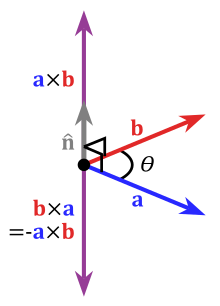
Value

Returns the generalized vector cross-product, a vector of length N.

Author(s)

Matthew Lundberg, in a [Stack Overflow post][https://stackoverflow.com/questions/36798301/r-compute-cross-product-of-vectors-physics]

Examples

xprod(1:3, 4:6)

# This works for an dimension
xprod(c(0,1))             # 2d
xprod(c(1,0,0), c(0,1,0)) # 3d
xprod(c(1,1,1), c(0,1,0)) # 3d
xprod(c(1,0,0,0), c(0,1,0,0), c(0,0,1,0)) # 4d