| Type: | Package |
| Title: | Tools for Calculating Hypocycloids, Epicycloids, Hypotrochoids, and Epitrochoids |
| Version: | 1.0.2 |
| Date: | 2023-08-29 |
| Author: | Peter Biber |
| Maintainer: | Peter Biber <castor.fiber@gmx.de> |
| Description: | Tools for calculating coordinate representations of hypocycloids, epicyloids, hypotrochoids, and epitrochoids (altogether called 'cycloids' here) with different scaling and positioning options. The cycloids can be visualised with any appropriate graphics function in R. |
| License: | GPL-3 |
| Collate: | 'ZFunktionen.r' |
| Encoding: | UTF-8 |
| NeedsCompilation: | no |
| Packaged: | 2023-08-29 10:05:30 UTC; casto |
| Repository: | CRAN |
| Date/Publication: | 2023-08-29 10:30:02 UTC |
Calculating coordinate representations of hypocycloids, epicyloids, hypotrochoids, and epitrochoids
Description
Functions for calculating coordinate representations of hypocycloids, epicyloids, hypotrochoids, and epitrochoids (altogether called 'cycloids' here) with different scaling and positioning options. The cycloids can be visualised with any appropriate graphics function in R.
Details
This package has been written for calculating cartesian coordinate
representations of hypocycloids, epicyloids, hypotrochoids, and
epitrochoids (altogether called 'cycloids' here). These can be
easily visualized with any R graphic routine that
handles two-dimensional data. All examples shown here use
standard R graphics. While there are technical applications, the
main purpose of this package is to create mathematical artwork.
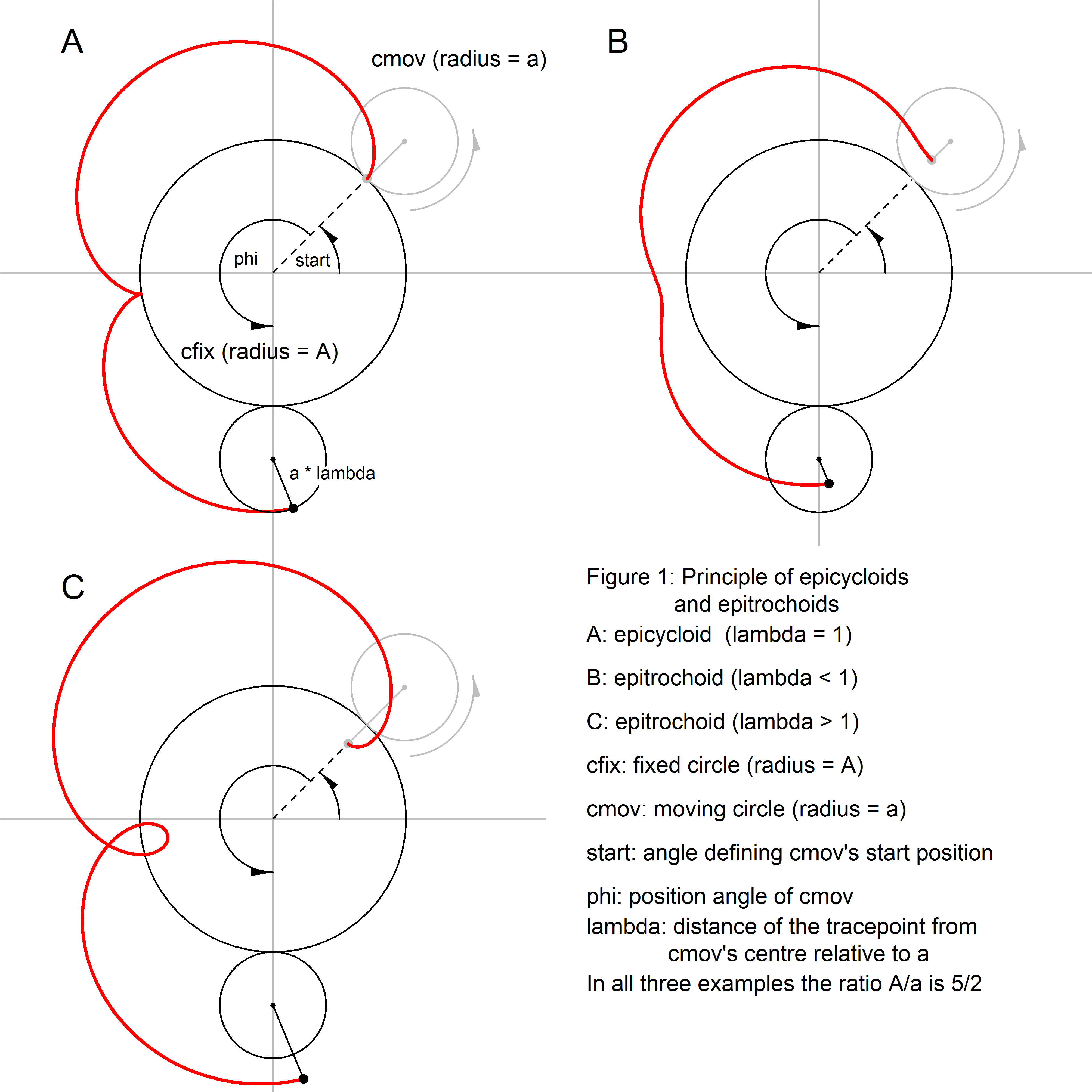
Geometrically, cycloids in the sense of this package are generated as
follows (Figure 1, 2): Imagine a circle cfix, with radius
A, which is fixed on a plane. Another circle, cmov,
with radius a, is rolling along cfix's circumference
at the outside of cfix. The figure created by the trace of
a point on cmov's circumference is called an epicycloid (Figure 1A).
If cmov is rolling not at the outside but at the inside of
cfix, the trace of a point on cmov's circumference
is called a hypocycloid (Figure 2A).
If in both cases the tracepoint is not located on
cmov's circumference but at a fixed distance from its midpoint
either in- or outside cmov, the resulting figure is an epitrochoid (Figure 1B, C)
or a hypotrochoid (Figure 2B, C), respectively. Hypotrochoids and epitrochoids
became quite popular through toys like the spirograph.
The most important functions of the package are
zykloid, zykloid.scaleA,
zykloid.scaleAa, and zykloid.scaleP.

Note
Type demo(cycloids) for seeing some examples.
Author(s)
Peter Biber
Maintainer: Peter Biber <castor.fiber@gmx.de>
References
Bronstein IN, Semendjaev KA, Musiol G, Muehlig H (2001): Taschenbuch der
Mathematik, 5th Edition, Verlag Harri Deutsch, 1186 p. (103 – 105)
http://en.wikipedia.org/wiki/Epicycloid
http://en.wikipedia.org/wiki/Hypocycloid
http://en.wikipedia.org/wiki/Epitrochoid
http://en.wikipedia.org/wiki/Hypotrochoid
http://en.wikipedia.org/wiki/Spirograph
See Also
zykloid, zykloid.scaleA,
zykloid.scaleAa, zykloid.scaleP
Examples
library(cycloids)

# Create and plot a hypocycloid, a hypotrochoid, an epicycloid,
# and an epitrochoid, all of them with radii A = 5 and a = 3
npeaks(5, 3)  # The cycloids will have five peaks
# The hypocycloid
cyc <- zykloid(A = 5, a = 3, lambda = 1, hypo = TRUE)
plot(y ~ x, data = cyc, type = "l", asp = 1, xlim = c(-12, 12),
     ylim = c(-12, 12), main = "A = 5, a = 3")
# The hypotrochoid
cyc <- zykloid(A = 5, a = 3, lambda = 1/2, hypo = TRUE)
lines(y ~ x, data = cyc, type = "l", asp = 1, col = "green")
# The epicycloid
cyc <- zykloid(A = 5, a = 3, lambda = 1, hypo = FALSE)
lines(y ~ x, data = cyc, type = "l", col = "red")
# The epitrochoid
cyc <- zykloid(A = 5, a = 3, lambda = 1/2, hypo = FALSE)
lines(y ~ x, data = cyc, type = "l", col = "blue")
legend("topleft", c("hypocycloid", "hypotrochoid", "epicycloid",
       "epitrochoid"), lty = rep("solid", 4),
       col = c("black", "green", "red", "blue"), bty = "n")


# Same Framework, different shape: A = 17, a = 5
npeaks(17, 5)  # The cycloids will have seventeen peaks
# The hypocycloid
cyc <- zykloid(A = 17, a = 5, lambda = 1, hypo = TRUE)
plot(y ~ x, data = cyc, type = "l", asp = 1, xlim = c(-27, 27),
     ylim = c(-27, 27), main = "A = 17, a = 5")
# The hypotrochoid
cyc <- zykloid(A = 17, a = 5, lambda = 1/2, hypo = TRUE)
lines(y ~ x, data = cyc, type = "l", asp = 1, col = "green")
# The epicycloid
cyc <- zykloid(A = 17, a = 5, lambda = 1, hypo = FALSE)
lines(y ~ x, data = cyc, type = "l", col = "red")
# The epitrochoid
cyc <- zykloid(A = 17, a = 5, lambda = 1/2, hypo = FALSE)
lines(y ~ x, data = cyc, type = "l", col = "blue")
legend("topleft", c("hypocycloid", "hypotrochoid", "epicycloid",
       "epitrochoid"), lty = rep("solid", 4),
       col = c("black", "green", "red", "blue"), bty = "n")


# Pretty - a classic Spirograph pattern with the same settings
# for A (5) and a (3) as in the first example.
# Varying parameters (here: lambda) within a loop often gives
# nice results.
op <- par(mar = c(0,0,0,0)) # no plot margins
lambdax <- seq(0.85, by = -0.05, length.out = 14)
ccol <- rep(c("blue", "blue", "red", "red"), 4)
plot.new()
plot.window(asp = 1, xlim = c(-4.5, 4.5), ylim = c(-4.5, 4.5))
# draw fourteen hypotrochoids with decreasing lambda
for (i in c(1:14)) {
     z <- zykloid(5, 3, lambdax[i])
     lines(y ~ x, data = z, type = "l", col = ccol[i])
} # for i
par(op) # set graphics parameters back to original values


# A bit more of the same kind to get the big picture...
op <- par(mar = c(0,0,0,0)) # no plot margins
lambdax <- seq(1, by = -0.05, length.out = 16)
ccol <- rep(c("blue", "blue", "red", "red"), 4)
plot.new()
plot.window(asp = 1, xlim = c(-11, 11), ylim = c(-11, 11))
# first loop: sixteen epitrochoids with decreasing lambda
for (i in 1:16) {
     z <- zykloid(5, 3, lambdax[i], hypo = FALSE)
     lines(y ~ x, data = z, type = "l", col = ccol[i])
} # for i - first loop
# first loop: sixteen epitrochoids with decreasing lambda
for (i in 1:16) {
     z <- zykloid(5, 3, lambdax[i], hypo = TRUE)
     lines(y ~ x, data = z, type = "l", col = ccol[i])
} # for i - second loop
par(op) # set graphics parameters back to original values


# Show off with an example for zykloid.scaleP
#    No plot margins, and ... paint it black
op <- par(mar = c(0,0,0,0), bg = "black")
lambdax <- seq(2, 0.0, -0.05) # Note: some lambdas are greater than 1
ccol <- rep(c("lightblue", "lightblue", "yellow", "yellow", "yellow"), 9)
plot.new()
plot.window(asp = 1, xlim = c(-1, 1), ylim = c(-1, 1))
for (ll in c(1:length(lambdax))) {
     z <- zykloid.scaleP(A = 7, a = 5, hypo = TRUE, lambda = lambdax[ll])
     lines(y ~ x, data = z, col = ccol[ll])
} # for ll
par(op) # set graphics parameters back to original values


# Spiky Flower with zykloid.scaleA and zykloid
op <- par(mar = c(0,0,0,0), bg = "black")
plot.new()
plot.window(asp = 1, xlim = c(-150, 150), ylim = c(-150, 150))
z <- zykloid.scaleA(A = 90, a = 32, lambda = 1, Radius = 150, hypo = TRUE)
lines(y ~ x, data = z, col = "lightblue")
for (ll in seq(2, 0.8, -0.4)) {
     if (ll == 2) ccol <- "royalblue"
     else         ccol <- "plum"
     z <- zykloid(A = 90, a = 32, lambda = ll, hypo = TRUE, steps = 360, start = pi/2)
     lines(y ~ x, data = z, col = ccol)
} # for ll
par(op)
Calculates the greatest common divisor of two natural numbers a and b based on the Euclidean Algorithm
Description
The function ggT calculates the greatest common divisor of two
natural numbers. In this package it is called by the function
kgV which calculates the least common multiple of
two natural numbers. The latter is needed by the function
zykloid and by the function npeaks
which calculates the number of peaks (or loops) a cycloid has.
As the greatest common divisor might be useful for other
purposes, the function ggT is accessible to external use in this
package.
Usage
ggT(a, b)
Arguments
a |
A natural number (integer value > 0) |
b |
A natural number (integer value > 0) |
Value
A natural number if a and b are natural numbers. In any other
case, the function returns NA.
Author(s)
Peter Biber
References
Bronstein IN, Semendjaev KA, Musiol G, Muehlig H (2001): Taschenbuch der
Mathematik, 5th Edition, Verlag Harri Deutsch, 1186 p. (p. 333)
http://en.wikipedia.org/wiki/Euclidean_algorithm
See Also
Examples
ggT(18, 6)        # 6
ggT(38, 105)      # 1
ggT(36, 9)        # 9
ggT(12, 9)        # 3
ggT(9, 12)        # 3
ggT(-5, 12)       # NA - only integer numbers > 0 allowed
ggT(3, 0)         # NA - only integer numbers > 0 allowed
ggT(3.2, 12)      # NA - only integer numbers > 0 allowed
Calculates the least common multiple of two natural numbers a and b
Description
The function kgV calculates the least common multiple of two natural
numbers. In this package it is used by the function zykloid
and by the function npeaks which calculates the
number of peaks (or loops) a cycloid has. As it might be useful
for other purposes, it is externally available in this package.
Usage
kgV(a, b)
Arguments
a |
A natural number (integer value > 0) |
b |
A natural number (integer value > 0) |
Value
A natural number if a and b are natural numbers. In any other
case, the function returns NA.
Author(s)
Peter Biber
References
Bronstein IN, Semendjaev KA, Musiol G, Muehlig H (2001): Taschenbuch der
Mathematik, 5th Edition, Verlag Harri Deutsch, 1186 p. (p. 334)
http://en.wikipedia.org/wiki/Least_common_multiple
See Also
Examples
kgV(18, 6)          #   18
kgV(38, 105)        # 3990
kgV(36, 9)          #   36
kgV(12, 9)          #   36
kgV(9, 12)          #   36
kgV(-5, 12)         # NA - only integer numbers > 0 allowed
kgV(3, 0)           # NA - only integer numbers > 0 allowed
kgV(3.2, 12)        # NA - only integer numbers > 0 allowed
Calculates the number of a cycloid's peaks based on the radii A (fixed circle) and a (moving circle)
Description
This function may be useful for calculating the number n of peaks
a cycloid (zykloid) based on the radii A (fixed
circle) and a (moving circle) will have. The equation for n is
n = kgV(A, a)/a
where kgV(A, a) is the least common multiple of A and a as
implemented in the function kgV
Usage
npeaks(A, a)
Arguments
A |
A natural number (integer value > 0) |
a |
A natural number (integer value > 0) |
Value
A natural number if A and a are natural numbers. In any other
case, the function returns NA.
Author(s)
Peter Biber
See Also
Examples
npeaks(18, 6)      #  3
npeaks(38, 105)    # 38
npeaks(36, 9)      #  4
npeaks(12, 9)      #  4
npeaks(9, 12)      #  3
npeaks(-5, 12)     # NA - only integer numbers > 0 allowed
npeaks(3, 0)       # NA - only integer numbers > 0 allowed
npeaks(3.2, 12)    # NA - only integer numbers > 0 allowed
Core function for calculating coordinate representations of hypocycloids, epicyloids, hypotrochoids, and epitrochoids (altogether called 'cycloids' here)
Description
This is the package's core function for calculating cycloids.
These are represented by a set of two-dimensional point
coordinates. Although this function provides the essential
mathematics, you may want to use the wrappers zykloid.scaleA,
zykloid.scaleAa, and zykloid.scaleP
due to their convenient scaling and positioning options.
Usage
zykloid(A, a, lambda, hypo = TRUE, steps = 360, start = pi/2)
Arguments
A |
The Radius of the fixed circle |
a |
The radius of the moving circle |
lambda |
The distance of the tracepoint from the moving circle's ( |
hypo |
logical. If TRUE, the resulting figure is a hypocycloid ( |
steps |
positive integer. The number of steps per circuit of the moving
circle ( |
start |
Start angle (radians) of the moving circle's ( |
Details
Geometrically, cycloids in the sense of this package are generated as
follows (Figure 1, 2): Imagine a circle cfix, with radius A,
which is fixed on a plane. Another circle, cmov, with radius
a, is rolling along cfix's circumference at the outside
of cfix. The figure created by the trace of a point on
cmov's circumference is called an epicycloid (Figure 1A).
If cmov is rolling not at the outside but at the inside of
cfix, the trace of a point on cmov's circumference
is called an hypocycloid (Figure 2A).
If in both cases the tracepoint is not located on cmov's
circumference but at a fixed distance from its midpoint
either in- or outside cmov, the resulting figure is an
epitrochoid (Figure 1B, C) or a hypotrochoid (Figure 2B, C),
respectively.
With the arguments of zykloid as defined above, the centre of cfix
in the origin, and phi being the counterclockwise angle of
cmov's midpoint against the start position with cfix'
centre as the pivot, the cartesian coordinates of a point on the
cycloid are calculated as follows:
x = (A + a) * cos(phi + start) - lambda * a * cos((A + a)/a * phi + start)
y = (A + a) * sin(phi + start) - lambda * a * sin((A + a)/a * phi + start)
Value
A dataframe with the columns x and y. Each row
represents a tracepoint position. The positions are ordered along
the trace with the last and the first point being identical in
order to warrant a closed figure when plotting the data.
Author(s)
Peter Biber
References
Bronstein IN, Semendjaev KA, Musiol G, Muehlig H (2001): Taschenbuch
der Mathematik, 5th Edition, Verlag Harri Deutsch, 1186 p.
(103 - 105)
http://en.wikipedia.org/wiki/Epicycloid
http://en.wikipedia.org/wiki/Hypocycloid
http://en.wikipedia.org/wiki/Epitrochoid
http://en.wikipedia.org/wiki/Hypotrochoid
See Also
zykloid.scaleA,
zykloid.scaleAa, zykloid.scaleP
Examples
# Very simple example
cycl <- zykloid(A = 17, a = 9, lambda = 0.9, hypo = TRUE)
plot(y ~ x, data = cycl, asp = 1, type = "l")


# More complex: Looks like a passion flower
op <- par(mar = c(0,0,0,0), bg = "black")
plot.new()
plot.window(asp = 1, xlim = c(-23, 23), ylim = c(-23, 23))
ll   <- seq(2, 0, -0.2)
ccol <- rep(c("lightblue", "lightgreen", "yellow", "yellow",
              "yellow"), 2)
for (i in c(1:length(ll))) {
     z <- zykloid(A = 15, a = 7, lambda = ll[i], hypo = TRUE)
     lines(y ~ x, data = z, col = ccol[i])
} # for i
par(op)


# Dense hypotrochoids
op <- par(mar = c(0,0,0,0), bg = "black")
plot.new()
plot.window(asp = 1, xlim = c(-1.5, 1.5), ylim = c(-1.5, 1.5))
m <- zykloid(A = 90, a = 89, lambda = 0.01)
lines(y ~ x, data = m, col = "grey")
m <- zykloid(A = 90, a = 89, lambda = 0.02)
lines(y ~ x, data = m, col = "red")
m <- zykloid(A = 90, a = 89, lambda = 0.015)
lines(y ~ x, data = m, col = "blue")
par(op)


# Fragile star
op <- par(mar = c(0,0,0,0), bg = "black")
plot.new()
plot.window(asp = 1, xlim = c(-14, 14), ylim = c(-14, 14))
l.max <- 1.6
l.min <- 0.1
ll <- seq(l.max, l.min, by = -1 * (l.max - l.min)/30)
n  <- length(ll)
ccol <- rainbow(n, start = 2/3, end = 1)
for (i in c(1:n)) {
    m <- zykloid(A = 9, a = 8, lambda = ll[i])
    lines(y ~ x, data = m, type = "l", col = ccol[i])
}  # for i
par(op)
Wrapper for zykloid which allows to scale and position
a cycloid by the radius A of the fixed circle and its midpoint
Description
While zykloid provides the basic functionality for
calculating cycloids, this functions allows to re-size a cycloid
by freely setting the radius on the fixed circle. In addition,
the cycloid can be re-positioned by locating the fix circle's
midpoint. See Figures 1 and 2 and zykloid for the
geometrical principles of cycloids.
Usage
zykloid.scaleA(A, a, lambda, hypo = TRUE, Cx = 0, Cy = 0,
               RadiusA = 1, steps = 360, start = pi/2)
Arguments
A |
The Radius of the fixed circle before re-sizing. Must be an integer
Number > 0. Together with |
a |
The radius of the moving circle before re-sizing. Must be an
integer Number > 0. Together with |
lambda |
The distance of the tracepoint from the moving circle's (c |
hypo |
logical. If TRUE, the resulting figure is a hypocycloid ( |
Cx |
x-coordinate of the fixed circle's midpoint. Default is 0. |
Cy |
y-coordinate of the fixed circle's midpoint. Default is 0. |
RadiusA |
The actual radius of the fixed circle. Default is 1. |
steps |
positive integer. The number of steps per circuit of the moving
circle ( |
start |
Start angle (radians) of the moving circle's ( |
Details
Value
A dataframe with the columns x and y. Each row represents a
tracepoint position. The positions are ordered along the trace
with the last and the first point being identical in order to
warrant a closed figure when plotting the data.
Author(s)
Peter Biber
See Also
zykloid,
zykloid.scaleAa, zykloid.scaleP
Examples
# Same hypotrochoid scaled to different radii of the fix circle
cycl1 <- zykloid.scaleA(A = 7, a = 3, lambda = 2/3, RadiusA = 1.3)
cycl2 <- zykloid.scaleA(A = 7, a = 3, lambda = 2/3, RadiusA = 1.0)
cycl3 <- zykloid.scaleA(A = 7, a = 3, lambda = 2/3, RadiusA = 0.7)
plot (y ~ x, data = cycl1, asp = 1, col = "red", type = "l",
      main = "A = 7, a = 3, lambda = 2/3")
lines(y ~ x, data = cycl2, asp = 1, col = "green")
lines(y ~ x, data = cycl3, asp = 1, col = "blue")
legend("topleft", c("RadiusA = 1.3", "RadiusA = 1.0", "RadiusA = 0.7"),
       lty = rep("solid", 3), col = c("red", "green", "blue"), bty = "n")


# In this example, RadiusA depends on the cosine of the x-coordinate
# of the fixed circle's centre
op <- par(mar = c(0,0,0,0), bg = "black")
ctrx <- seq(-2*pi, 2*pi, pi/10)
ccol <- rainbow(length(ctrx))
plot.new()
plot.window(asp = 1, xlim = c(-8, 8), ylim = c(-0.5, 0.5))
for(i in c(1:length(ctrx))) {
    zzz <- zykloid.scaleA(A = 9, a = 7, hypo = TRUE, Cx = ctrx[i],
                          Cy = -ctrx[i], lambda = 0.9,
                          RadiusA = 1.5 + cos(ctrx[i]), start = -pi/4)
    lines(y ~ x, data = zzz, col = ccol[i])
} # for i
par(op)


# Geometric degression of RadiusA makes a nice star
op <- par(mar = c(0,0,0,0), bg = "black")
plot.new()
plot.window(asp = 1, xlim = c(-10, 10), ylim = c(-10, 10))
rad <- 10
n <- 60
ccol <- heat.colors(n)
for(i in c(1:n)) {
    if (i/2 != floor(i/2)) { sstart = pi/2 }
    else                   { sstart = pi/4 }
    zzz <- zykloid.scaleA(A = 4, a = 3, RadiusA = rad, lambda = 1,
                          start = sstart)
    lines(y ~ x, data = zzz, col = ccol[i])
    rad <- rad * 0.9
} # for i
par(op)


# A windmill
op <- par(mar = c(0,0,0,0), bg = "black")
plot.new()
plot.window(asp = 1, xlim = c(-1.4, 1.4), ylim = c(-1.4, 1.4))
rrad <- sqrt(seq(0.1, 2, 0.1))
n    <- length(rrad)
ccol <- rainbow(n, start = 0, end = 0.3)
for(i in c(1:n)) {
    zzz <- zykloid.scaleA(A = 7, a = 3, RadiusA = rrad[i],
           hypo = TRUE, lambda = 1.1,
           start = pi/2 - (1*pi/7 - (i - 1) * 2*pi/(7 * n)))
    lines(y ~ x, data = zzz, col = ccol[n + 1 - i])
} # for i
par(op)


# Advanced Example: A series of cycloids with their centres
# located on a logarithmic spiral
op <- par(mar = c(0,0,0,0), bg = "black")
plot.new()
plot.window(asp = 1, xlim = c(-50, 50), ylim = c(-50, 50))
a     <- 1/32     # spiral's scaling constant
alpha <- pi/20    # spiral's slope angle
sphi  <- seq(0, 18 * pi, pi/25)   # series of angles for cycloid centres
rad  <- a * exp(tan(alpha)*sphi)  # corresponding spiral radii
spx  <- rad * cos(sphi)           # corresponding x-coordinates
spy  <- rad *sin(sphi)            # corresponding y-coordinates
n    <- length(sphi)
ccol <- rainbow(n, start = 2/3, end = 1/2)
for (i in c(1:n)) {
     czc <- zykloid.scaleA(A = 3, a = 1, lambda = 1.5,
            Cx = spx[i], Cy = spy[i],
            RadiusA = rad[i]/2.5, # cycloid radii depends on spiral radii
            start = pi + sphi[i]) # angle cycloid towards spiral centre
     lines(y ~ x, data = czc, col = ccol[i])
} # for i
par(op)
Wrapper for zykloid which scales a cycloid by its
outer radius and allows free positioning
Description
While zykloid provides the basic functionality for
calculating cycloids, this functions allows to re-size a cycloid
by freely setting the radius of its circumcircle. In addition,
the cycloid can be re-positioned by locating the fixed circle's
midpoint. This function behaves similarly as zykloid.scaleP.
See details. Figures 1 and 2 and zykloid describe the
geometrical principles of cycloids.
Usage
zykloid.scaleAa(A, a, lambda, hypo = TRUE, Cx = 0, Cy = 0,
                RadiusAa = 1, steps = 360, start = pi/2)
Arguments
A |
The Radius of the fixed circle before re-sizing. Must be an integer
Number > 0. Together with |
a |
The radius of the moving circle before re-sizing. Must be an
integer Number > 0. Together with |
lambda |
The distance of the tracepoint from the moving circle's ( |
hypo |
logical. If TRUE, the resulting figure is a hypocycloid ( |
Cx |
x-coordinate of the fixed circle's midpoint. Default is 0. |
Cy |
y-coordinate of the fixed circle's midpoint. Default is 0. |
RadiusAa |
The actual radius of the cycloids outer circle. Default is 1. |
steps |
positive integer. The number of steps per circuit of the moving circle (cmov) for which tracepoint positions are calculated. The default, 360, means steps of 1 degree for the movement of cmov. Analogously, steps = 720 would mean steps of 0.5 degrees. |
start |
Start angle (radians) of the moving circle's ( |
Details
This function scales in either case the radius of the whole
cycloid's circumcircle. Thus, for hypocycloids and hypotrochoids
it will behave the same way as zykloid.scaleP.
For epicycloids and epitrochoids their output will be different.
zykloid.scaleAa scales the outer edge of the figure, while
zykloid.scaleP always scales the circle where the
peaks of the figure are located on. In the case of epicycloids
and epitrochoids this is at the inside of the figure (see
examples).
Figure 1 and 2 show the principle behind cycloid construction:
Value
A dataframe with the columns x and y. Each row represents
a tracepoint position. The positions are ordered along the trace
with the last and the first point being identical in order to
warrant a closed figure when plotting the data.
Author(s)
Peter Biber
See Also
zykloid,
zykloid.scaleA, zykloid.scaleP
Examples
# Same epicycloid scaled to different maximum radii of the figure
cycl1 <- zykloid.scaleAa(A = 21, a = 11, lambda = 1, hypo = FALSE,
                         RadiusAa = 100)
cycl2 <- zykloid.scaleAa(A = 21, a = 11, lambda = 1, hypo = FALSE,
                         RadiusAa =  70)
cycl3 <- zykloid.scaleAa(A = 21, a = 11, lambda = 1, hypo = FALSE,
                         RadiusAa =  40)
plot (y ~ x, data = cycl1, col = "red", asp = 1, type = "l",
      main = "A = 21, a = 11, lambda = 1")
lines(y ~ x, data = cycl2, col = "green")
lines(y ~ x, data = cycl3, col = "blue")
legend("topleft", c("RadiusAa = 100", "RadiusAa =  70", "RadiusAa =  40"),
       lty = rep("solid", 3), col = c("red", "green", "blue"), bty = "n")


# Pentagram by constructing a hypocycloid and an epicycloid
# with the same outer radius and scaling this radius exponentially
op <- par(mar = c(0,0,0,0), bg = "black")
plot.new()
plot.window(asp = 1, xlim = c(-40, 40), ylim = c(-40, 40))
n <- 20
ccol <- heat.colors(n)
for(i in c(1:n)) {
    zzz <- zykloid.scaleAa(A = 5, a = 2,
           RadiusAa = 38*exp(-0.05*(i-1)), hypo = FALSE, lambda = 1)
    lines(y ~ x, data = zzz, col = ccol[i])
    zzz <- zykloid.scaleAa(A = 5, a = 2,
           RadiusAa = 38*exp(-0.05*(i-1)), hypo = TRUE,  lambda = 1)
    lines(y ~ x, data = zzz, col = ccol[i])
} # for i
par(op)


# Psychedelic star by modifying lambda while keeping the outer
# radius constant
op <- par(mar = c(0,0,0,0), bg = "black")
plot.new()
plot.window(asp = 1, xlim = c(-5, 5), ylim = c(-5, 5))
llam <- seq(0, 8, 0.2)
ccol <- terrain.colors(length(llam))
for(i in c(1:length(llam))) {
    zzz <- zykloid.scaleAa(A = 5, a = 1, RadiusAa = 4.5,
           hypo = FALSE, lambda = llam[i])
    lines(y ~ x, data = zzz, col = ccol[i])
} # for i
par(op)
Wrapper for zykloid which scales a cycloid by the
circle its peaks are located on and allows free positioning
Description
While zykloid provides the basic functionality for
calculating cycloids, this functions allows to re-size a cycloid
by freely setting the radius of the circle its peaks are located
on. In addition, the cycloid can be re-positioned by locating
the fixed circle's midpoint. This function behaves similarly as
zykloid.scaleAa. See details. See Figures 1, 2, and
zykloid for the geometrical principles of cycloids.
Usage
zykloid.scaleP(A, a, lambda, hypo = TRUE, Cx = 0, Cy = 0,
               RadiusP = 1, steps = 360, start = pi/2)
Arguments
A |
The Radius of the fix circle before re-sizing. Must be an integer
Number > 0. Together with |
a |
The radius of the moving circle before re-sizing. Must be an
integer Number > 0. Together with |
lambda |
The distance of the tracepoint from the moving circle's ( |
hypo |
logical. If TRUE, the resulting figure is a hypocycloid ( |
Cx |
x-coordinate of the fix circle's midpoint. Default is 0. |
Cy |
y-coordinate of the fix circle's midpoint. Default is 0. |
RadiusP |
The actual radius of the circle the cycloid's peaks are located on. Default is 1. |
steps |
positive integer. The number of steps per circuit of the moving
circle ( |
start |
Start angle (radians) of the moving circle's ( |
Details
This function scales the radius of the circle the cycloids peaks
are located on. For hypocycloids and hypotrochoids it will thus
behave the same way as zykloid.scaleAa. For
epicycloids and epitrochoids the output will be different.
While zykloid.scaleAa scales the outer edge of the
figure, zykloid.scaleP always scales the circle where the
peaks of the figure are located on. In the case of epicycloids
and epitrochoids this is at the inside of the figure (see
examples below).
Figure 1 and 2 show the principle behind cycloid construction:
Value
A dataframe with the columns x and y. Each row represents
a tracepoint position. The positions are ordered along the trace
with the last and the first point being identical in order to
warrant a closed figure when plotting the data.
Author(s)
Peter Biber
See Also
zykloid,
zykloid.scaleA, zykloid.scaleAa
Examples
# Epitrochoids with different lambda scaled to the same radius of
# the peak circle
cycl1 <- zykloid.scaleP(A = 21, a = 11, lambda = 1.2, hypo = FALSE,
                         RadiusP = 10)
cycl2 <- zykloid.scaleP(A = 21, a = 11, lambda = 1.0, hypo = FALSE,
                         RadiusP = 10)
cycl3 <- zykloid.scaleP(A = 21, a = 11, lambda = 0.8, hypo = FALSE,
                         RadiusP = 10)
plot (y ~ x, data = cycl1, col = "red", asp = 1, type = "l",
      main = "A = 21, a = 11, RadiusP = 10")
lines(y ~ x, data = cycl2, col = "green")
lines(y ~ x, data = cycl3, col = "blue")
legend("topleft", c("lambda = 1.2", "lambda =  1.0", "lambda =  0.8"),
       lty = rep("solid", 3), col = c("red", "green", "blue"),
       bty = "n")


# Cool Disk by scaling the start angle with an
# exponential function ...
op <- par(mar = c(0,0,0,0), bg = "black")
plot.new()
plot.window(asp = 1, xlim = c(-11, 11), ylim = c(-11, 11))
n <- 30
ccol <- topo.colors(n)
for(i in c(1:n)) {
    zzz <- zykloid.scaleP(A = 3, a = 1, RadiusP = 6, lambda = 1,
           start = 2*pi/3 * exp(-0.1 * (i - 1)), hypo = FALSE)
    lines(y ~ x, data = zzz, col = ccol[i])
} # for i
par(op)


# ... the free space in the centre could be filled with
# the corresponding hypocycloid ...
op <- par(mar = c(0,0,0,0), bg = "black")
plot.new()
plot.window(asp = 1, xlim = c(-11, 11), ylim = c(-11, 11))
n <- 30
ccol <- topo.colors(n)
for(i in c(1:n)) {
    zzz <- zykloid.scaleP(A = 3, a = 1, RadiusP = 6, lambda = 1,
           start = 2*pi/3 * exp(-0.1 * (i - 1)), hypo = FALSE)
    lines(y ~ x, data = zzz, col = ccol[i])
    zzz <- zykloid.scaleP(A = 3, a = 1, RadiusP = 6, lambda = 1,
           start = 2*pi/3 * exp(-0.1 * (i - 1)), hypo = TRUE)
    lines(y ~ x, data = zzz, col = ccol[i])
} # for i
par(op)


# ... or the same ring again and again.
op <- par(mar = c(0,0,0,0), bg = "black")
plot.new()
plot.window(asp = 1, xlim = c(-11, 11), ylim = c(-11, 11))
n <- 30
ccol <- topo.colors(n)
rad <- 6
for(g in c(1:7)) {
    for(i in c(1:n)) {
        zzz <- zykloid.scaleP(A = 3, a = 1, RadiusP = rad,
               lambda = 1, start = 2*pi/3 * exp(-0.1 * (i - 1)),
               hypo = FALSE)
        lines(y ~ x, data = zzz, col = ccol[i])
    } # for i
    rad <- rad * 3/5
} # for g
par(op)


# Cauliflower pattern. Here, an exponential function is used
# for scaling the radius of the circle the cycloid's loops
# are on.
op <- par(mar = c(0,0,0,0), bg = "black")
plot.new()
plot.window(asp = 1, xlim = c(-22, 22), ylim = c(-22, 22))
n <- 15
dcol <- heat.colors(n)
for(i in c(1:n)) {
    lambdax <- seq(2.0, 2.2, 0.1)
    for(j in c(1:length(lambdax))) {
        zzz <- zykloid.scaleP(A = 11, a = 1,
               RadiusP = 15 * exp(-0.3 * (i - 1)),
               lambda = lambdax[j], hypo = FALSE,
               start = pi/2 + (i - 1)*pi/11)
        if(j/2 == floor(j/2)) { colx <- "blue" }
        else                  { colx <- dcol[n + 1 - i] }
        lines(y ~ x, data = zzz, col = colx)
    } # for j
} # for i
par(op)


# Sparkling star
op <- par(mar = c(0,0,0,0), bg = "black")
plot.new()
plot.window(asp = 1, xlim = c(-15, 15), ylim = c(-15, 15))
llam <- seq(0, 8, 0.2)
ccol <- rainbow(length(llam), start = 2/3, end = 1/3)
for(i in c(1:length(llam))) {
    zzz <- zykloid.scaleP(A = 5, a = 1, RadiusP = 2.1,
           hypo = FALSE, lambda = llam[i], start = pi/5)
    lines(y ~ x, data = zzz, col = ccol[i])
} # for i
par(op)