
Statistical theory incorrectly states that the Wilcoxon-Mann-Whitney (WMW) test examines \(\mathrm{H_0\colon F = G}\). We demonstrate this theoretical claim is untenable: the WMW statistic, when standardized, is the empirical AUC (eAUC), which measures \(P(X < Y)\) and cannot detect distributional equality. Through Monte Carlo analysis of zero-mean heteroscedastic Gaussians and corresponding asymptotic theory, we show that WMW tests \(\mathrm{H_0\colon AUC = 0.5}\) (no systematic discrimination) rather than distributional equality. Moreover, the traditional alternative hypothesis of stochastic dominance is unnecessarily restrictive; WMW is consistent against the broader alternative \(\mathrm{H_1\colon AUC \neq 0.5}\), as established by Van Dantzig (1951). We provide theoretical framework and implementation consistent with what the WMW eAUC statistic actually computes, including tie-corrected asymptotics and finite-sample bias corrections. For detalis, see (Grendár 2025).
The primary goal of wmwAUC is to provide inferences for the Wilcoxon-Mann-Whitney test of \(\mathrm{H_0\colon AUC = 0.5}\). Besides the asymtotic inferences the library provides two variants of finite-sample bias correction:
Exact Unbiased (EU) Method: Universal approach handling data with arbitrary tie patterns through the mid-rank kernel and exact finite-sample unbiased variance estimation from Hoeffding decomposition theory. Reduces correctly to the continuous case when no ties are present.
Bias-Corrected (BC) Method: Alternative for continuous data without ties, using individual component bias correction with \(O(n^{-1})\) finite-sample corrections and Welch-Satterthwaite degrees of freedom. Assumes continuous distributions with no ties.
The EU method serves as the default implementation, providing:
Universal applicability (handles any data type - continuous, discrete, or mixed)
Exact finite-sample unbiasedness (not asymptotic approximation)
Theoretically principled tie handling through mid-rank kernel
The BC method is available for users specifically working with continuous data or requiring compatibility with traditional variance estimation approaches.
Key functions include:
wmw_test(): Main testing function using EU
methodology with option to use BC method for continuous-only
data
wmw_pvalue(): WMW AUC p-values for continuous data,
based on the BC method
wmw_pvalue_ties(): WMW AUC p-values for any type of
data, based on the EU method
pseudomedian_ci(): Confidence intervals for
Hodges-Lehmann pseudomedian
quadruplot(): Diagnostics for location shift
assumption
You can install the development version of wmwAUC using
devtools::install_github('grendar/wmwAUC')Consider the setting of two zero-mean different-scale gaussians. Then the traditional \(\mathrm{H_0\colon F = G}\) of WMW test is false and \(\mathrm{H_0\colon F \neq G}\) holds.
The Monte Carlo simulation demonstrates that the normalized test statistic \(U/(n_1n_2)\) which is just eAUC, concentrates asymptotically on 0.5 - the value expected under a true null hypothesis.
If WMW tested distributional equality, the test statistic should not concentrate on its null value when distributions clearly differ.
Also note that under \(\mathrm{H_0\colon F \neq G}\), p-values should concentrate near zero, yet the observed distribution is nearly uniform with a slightly elevated first bins, consistent with testing a true null hypothesis (\(\mathrm{H_0\colon AUC = 0.5}\)) using miscalibrated variance estimation.
#############################################################################
#
# Simulation 1: H0: F=G is erroneously too broad
#
#############################################################################
#
# This simulation takes several minutes to complete
# N = 10000
# n = 1000
# set.seed(123L)
# pval_wt = pval_wmw = eauc = numeric(N)
# for (i in 1:N) {
#
#   x = rnorm(n, sd = 0.1)
#   y = rnorm(n, sd = 3)
#   # wilcox.test() of H0: F = G
#   wt = wilcox.test(x, y)
#   pval_wt[i] = wt$p.value
#   # wmw_test() of H0: AUC = 0.5
#   pval_wmw[i] = wmw_pvalue(x, y)
#   # eAUC
#   eauc[i] = wt$statistic/(n*n)
#   #
# }
data(simulation1)  # List eauc, pval_wt, pval_wmw
#
Empirical AUC centered at 0.5 despite \(\mathrm{F \neq G}\).

Traditional p-values under \(\mathrm{H_1}\) should concentrate near 0.

Correct p-values for testing \(\mathrm{H_0\colon AUC = 0.5}\).
The two zero-mean different-scale gaussians setting does not satisfy the traditional \(\mathrm{H_1}\) of the stochastic dominance. But, as proved by Van Dantzig in 1951, WMW is consistent for broader \(\mathrm{H_1\colon AUC \neq 0.5}\).
#############################################################################
#
# Simulation 2: H1: F stoch. dominates G is too narrow
#               WMW is consistent for broader H1: AUC != 0.5
#
#############################################################################
#
#
# This simulation takes several minutes to complete
# N = 10000
# n = 1000
# set.seed(123L)
# pval_wt = pval_wmw = eauc = numeric(N)
# for (i in 1:N) {
# #
#   # gaussians with different location and scale
#   # does not satisfy stochastic dominance
#   x = rnorm(n, 0, sd = 0.1)
#   y = rnorm(n, 0.5, sd = 3)
#   # wilcox.test H0: F = G vs H1: (F stochastically dominates G) OR (G stochastically dominates F)
#   wt = wilcox.test(x, y)
#   pval_wt[i] = wt$p.value
#   # wmw_test H0: AUC = 0.5 vs H1: AUC neq 0.5
#   pval_wmw[i] = wmw_pvalue(x, y)
#   # eAUC
#   eauc[i] = wt$statistic/(n*n)
# #
# }
data(simulation2)  # List of eauc, pval_wt, pval_wmw
# WMW detects broader alternatives than traditional stochastic dominance


Confidence interval for the pseudomedian is obtained by inverting the
test; see pseudomedian_ci() for implementation that handles
the edge cases in the same way as wilcox.test().
In this simulation study, N = 500 MC replicates are created, of 300
samples from the standard normal distribution and 300 samples from the
Laplace distribution with location = 0, scale = 1. Properties of 95%
confidence intervals obtained under H0: AUC = 0.5 are compared with
those returned by wilcox.test().
# #############################################################################
# #
# # Simulation 3: confidence interval for pseudomedian derived under H0: AUC = 0.5
# #               MC study of N = 500 replicas
# #               x ~ rnorm(300, 0,1)
# #               y ~ rlaplace(300, 0,1)
# #
# #############################################################################
#
#
#
# This simulation takes long time to complete
# N <- 500
# n_test <- 300
#
# set.seed(123L)
# wmw_ci = wt_ci = list(N)
# eauc = pseudomed = numeric(N)
# for (i in 1:N) {
#  #
#  x_test <- rnorm(n_test, 0, 1)
#  y_test <- VGAM::rlaplace(n_test, 0, 1)
#
#  wmw_test <- pseudomedian_ci(x_test, y_test, conf.level = 0.9, pvalue_method = 'BC')
#  wmw_ci[[i]] = wmw_test$conf.int
#  wt_test <- wilcox.test(x_test, y_test, conf.int = TRUE)
#  wt_ci[[i]] = wt_test$conf.int
#  eauc[i] = wt_test$statistic/(n_test*n_test)
#  pseudomed[i] = as.numeric(wt_test$estimate)
#  #
# }
#
#
data(simulation3)  # List of wmw_ci, wt_ci, eauc, pseudomedian
#
# Average across MC of confidence intervals obtained under H0: AUC=0.5
colMeans(simulation3$wmw_ci)
#> [1] -0.1701256  0.1735400
# Average across MC of confidence intervals from wilcox.test()
colMeans(simulation3$wt_ci)
#> [1] -0.1754612  0.1790767
#
# Average across MC of eAUC
mean(simulation3$eauc)
#> [1] 0.5004063

# Coverage
length(which((simulation3$wmw_ci[,1] < 0) & (simulation3$wmw_ci[,2] > 0)))
#> [1] 470
length(which((simulation3$wt_ci[,1] < 0) & (simulation3$wt_ci[,2] > 0)))
#> [1] 473

# Mean pseudomedian
mean(simulation3$pseudomed)
#> [1] 0.001776475Real data analyzed by WMW test of no group discrimination.
data(gemR::MS)
da <- MS

# preparing data frame
class(da$proteins) <- setdiff(class(da$proteins), "AsIs")
df <- as.data.frame(da$proteins)
df$MS <- da$MSwmd <- wmw_test(P19099 ~ MS, data = df, ref_level = 'no')
wmd
#>
#> Wilcoxon-Mann-Whitney Test of No Group Discrimination
#>
#> data: P19099 by MS (n1 = 37, n2 = 64)
#> groups: yes vs no (reference)
#> U = 1726, eAUC = 0.729, p-value = 0.000007, method = EU
#> alternative hypothesis for AUC: two.sided
#> 95 percent confidence interval for AUC (hanley):
#> 0.623 0.835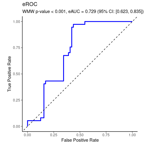
Synthetic data illustrating the special case of location shift assumption.
data(Ex2)
da <- Ex2

# WMW test
wmd <- wmw_test(y ~ group, data = da, ref_level = 'control')
wmd
#>
#>         Wilcoxon-Mann-Whitney Test of No Group Discrimination
#>
#> data: y by group (n1 = 100, n2 = 100)
#> groups: case vs control (reference)
#> U = 3705, eAUC = 0.370, p-value = 0.001106, method = EU
#> alternative hypothesis for AUC: two.sided
#> 95 percent confidence interval for AUC (hanley):
#>  0.294 0.447
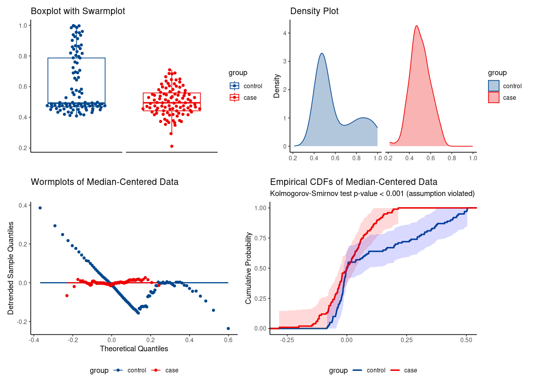 location-shift assumption not tenable.
Erroneous use of location-shift special case of WMW would falsely conclude significant median difference despite identical medians.
#>
#>         Wilcoxon-Mann-Whitney Test of No Group Discrimination
#>
#> data: y by group (n1 = 100, n2 = 100)
#> groups: case vs control (reference)
#> U = 3705, eAUC = 0.370, p-value = 0.001106, method = EU
#> alternative hypothesis for AUC: two.sided
#> 95 percent confidence interval for AUC (hanley):
#>  0.294 0.447
#>
#> Location-shift analysis (under F1(x) = F2(x - delta)):
#> alternative hypothesis for location: two.sided
#> Hodges-Lehmann median of all pairwise distances:
#>  -0.048 [location effect size: eAUC = 0.370]
#> 95 percent confidence interval for median of all pairwise distances:
#>  -0.084 -0.037
Indeed, the medians are essentially the same:
median(da$y[da$group == 'case'])
#> [1] 0.4949383
median(da$y[da$group == 'control'])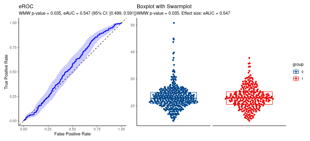
#> [1] 0.4926145WMW applied to another real-life data set.
data(wesdr)
da = wesdr
da$ret = as.factor(da$ret)
# WMW
wmd <- wmw_test(bmi ~ ret, data = da, ref_level = '0')
wmd
#>
#>         Wilcoxon-Mann-Whitney Test of No Group Discrimination
#>
#> data: bmi by ret (n1 = 278, n2 = 391)
#> groups: 1 vs 0 (reference)
#> U = 59417.5, eAUC = 0.547, p-value = 0.035168, method = EU
#> alternative hypothesis for AUC: two.sided
#> 95 percent confidence interval for AUC (hanley):
#>  0.502 0.591
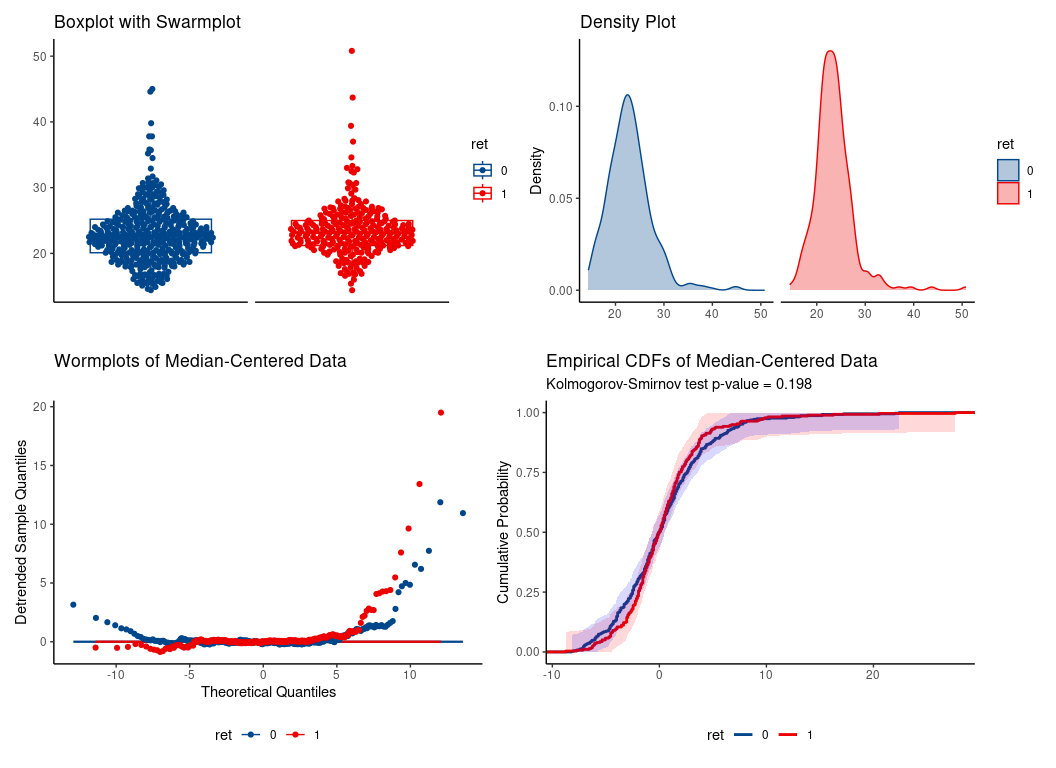 hence, location shift assumption is tenable.
wml <- wmw_test(bmi ~ ret, data = da, ref_level = '0',
                 ci_method = 'boot', special_case = TRUE, n_grid = 100)
wml
#>
#>         Wilcoxon-Mann-Whitney Test of No Group Discrimination
#>
#> data: bmi by ret (n1 = 278, n2 = 391)
#> groups: 1 vs 0 (reference)
#> U = 59417.5, eAUC = 0.547, p-value = 0.035168, method = EU
#> alternative hypothesis for AUC: two.sided
#> 95 percent confidence interval for AUC (boot):
#>  0.499 0.591
#>
#> Location-shift analysis (under F1(x) = F2(x - delta)):
#> alternative hypothesis for location: two.sided
#> Hodges-Lehmann median of all pairwise distances:
#>  0.600 [location effect size: eAUC = 0.547]
#> 95 percent confidence interval for median of all pairwise distances:
#>  0.294 0.906
Plot
AI-assisted code generation via Claude Pro by Anthropic was used in development. All generated content was verified, tested, and enhanced by the package author.