#spatialLIBD hashtag. You can find previous tweets that way as shown here. Thank you!
## Study design
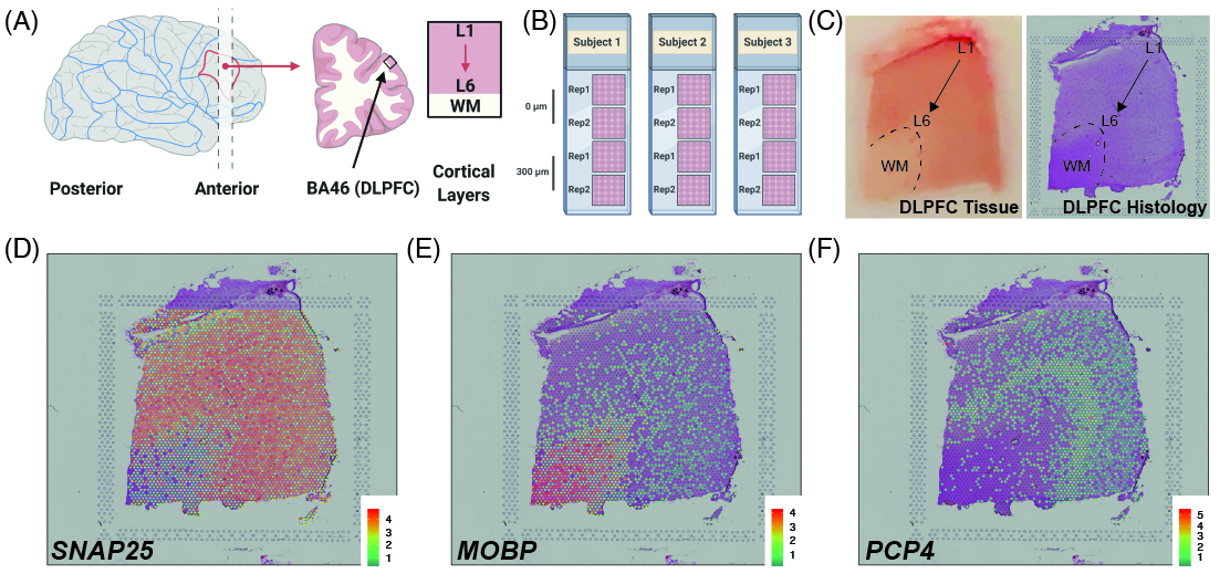
As a quick overview, the data presented here is from portion of the DLPFC that spans six neuronal layers plus white matter (**A**) for a total of three subjects with two pairs of spatially adjacent replicates (**B**). Each dissection of DLPFC was designed to span all six layers plus white matter (**C**). Using this web application you can explore the expression of known genes such as _SNAP25_ (**D**, a neuronal gene), _MOBP_ (**E**, an oligodendrocyte gene), and known layer markers from mouse studies such as _PCP4_ (**F**, a known layer 5 marker gene).
 ## Shiny website mirrors
* [Main shiny application website](http://spatial.libd.org/spatialLIBD)
* [Shinyapps](https://libd.shinyapps.io/spatialLIBD/)
# Basics
## Install `spatialLIBD`
`R` is an open-source statistical environment which can be easily modified to enhance its functionality via packages. `r Biocpkg('spatialLIBD')` is a `R` package available via Bioconductor. `R` can be installed on any operating system from [CRAN](https://cran.r-project.org/) after which you can install `r Biocpkg('spatialLIBD')` by using the following commands in your `R` session:
```{r 'install', eval = FALSE}
if (!requireNamespace("BiocManager", quietly = TRUE)) {
install.packages("BiocManager")
}
BiocManager::install("spatialLIBD")
## Check that you have a valid Bioconductor installation
BiocManager::valid()
```
To run all the code in this vignette, you might need to install other R/Bioconductor packages, which you can do with:
```{r "install_deps", eval = FALSE}
BiocManager::install("spatialLIBD", dependencies = TRUE, force = TRUE)
```
If you want to use the development version of `spatialLIBD`, you will need to use the R version corresponding to the current Bioconductor-devel branch as described in more detail on the [Bioconductor website](http://bioconductor.org/developers/how-to/useDevel/). Then you can install `spatialLIBD` from GitHub using the following command.
```{r "install_devel", eval = FALSE}
BiocManager::install("LieberInstitute/spatialLIBD")
```
## Required knowledge
`r Biocpkg('spatialLIBD')` `r Citep(bib[['spatialLIBD']])` is based on many other packages and in particular in those that have implemented the infrastructure needed for dealing with single cell RNA sequencing data, visualization functions, and interactive data exploration. That is, packages like `r Biocpkg('SingleCellExperiment')` that allow you to store the data, `r CRANpkg('ggplot2')` and `r CRANpkg('plotly')` for visualizing the data, and `r CRANpkg('shiny')` for building an interactive interface. A `r Biocpkg('spatialLIBD')` user who only accesses the web application is not expected to deal with those packages directly. A `r Biocpkg('spatialLIBD')` user will need to be familiar with `r Biocpkg('SingleCellExperiment')` and `r CRANpkg('ggplot2')` to understand the data provided by `r Biocpkg('spatialLIBD')` or the graphical results `r Biocpkg('spatialLIBD')` provides. Furthermore, it'll be useful for the user to know about `r CRANpkg('shiny')` and `r CRANpkg('plotly')` if you wish to adapt the web application provided by `r Biocpkg('spatialLIBD')`.
If you are asking yourself the question "Where do I start using Bioconductor?" you might be interested in [this blog post](http://lcolladotor.github.io/2014/10/16/startbioc/#.VkOKbq6rRuU).
## Asking for help
As package developers, we try to explain clearly how to use our packages and in which order to use the functions. But `R` and `Bioconductor` have a steep learning curve so it is critical to learn where to ask for help. The blog post quoted above mentions some but we would like to highlight the [Bioconductor support site](https://support.bioconductor.org/) as the main resource for getting help regarding Bioconductor. Other alternatives are available such as creating GitHub issues and tweeting. However, please note that if you want to receive help you should adhere to the [posting guidelines](http://www.bioconductor.org/help/support/posting-guide/). It is particularly critical that you provide a small reproducible example and your session information so package developers can track down the source of the error.
## Citing `spatialLIBD`
We hope that `r Biocpkg('spatialLIBD')` will be useful for your research. Please use the following information to cite the package and the research article describing the data provided by `r Biocpkg('spatialLIBD')`. Thank you!
```{r 'citation'}
## Citation info
citation("spatialLIBD")
```
# Overview
The `r Biocpkg('spatialLIBD')` `r Citep(bib[['spatialLIBD']])` package was developed for analyzing the human dorsolateral prefrontal cortex (DLPFC) spatial transcriptomics data generated with the 10x Genomics Visium technology by researchers at the Lieber Institute for Brain Development (LIBD) `r Citep(bib[['spatialLIBDpaper']])`. An initial `r CRANpkg('shiny')` application was developed for interactively exploring this data and for assigning human brain layer labels to the each spot for each sample generated. While this was useful enough for our project, we made this [Bioconductor](http://bioconductor.org/) package in case you want to:
* access our Visium data to get some data from this new technology and develop methods or infrastructure for other Visium datasets.
* re-shape your data into what ours is structured as, then re-use the visualization functions and/or the shiny app itself.
* want to explore our data in more detail. This can range from launching the `r CRANpkg('shiny')` application locally to diving into the specifics of the data from our project `r Citep(bib[['spatialLIBDpaper']])`.
In this vignette we'll showcase how you can access the Human DLPFC LIBD Visium dataset `r Citep(bib[['spatialLIBDpaper']])`, the R functions provided by `r Biocpkg('spatialLIBD')` `r Citep(bib[['spatialLIBD']])`, and an overview of how you can re-shape your own Visium dataset to match the structure we used.
To get started, please load the `r Biocpkg('spatialLIBD')` package.
```{r setup, message = FALSE, warning = FALSE}
library("spatialLIBD")
```
# Human DLPFC Visium dataset
The human DLPFC 10x Genomics Visium dataset analyzed by LIBD researchers and colleagues is described in detail by Maynard, Collado-Torres et al `r Citep(bib[['spatialLIBDpaper']])`. However, briefly, this dataset is composed of:
* Three brain subjects (all controls; two males, one female; ages 30-46; [details](https://github.com/LieberInstitute/HumanPilot/blob/master/Analysis/visium_dlpfc_pilot_sample_metrics.tsv)).
* Four images per subject: two spatially adjacent replicates at position 0, then two more spatially adjacent replicates 300 micrometers away.
* Slices designed to cover layers 1 through 6 and the white matter (WM) of the dorsolateral prefrontal cortex (DLPFC).
## Data specifics
We combined all the Visium data into a single `r Biocpkg('SpatialExperiment')` `r Citep(bib[['SpatialExperiment']])` object that we typically refer to as __`spe`__ ^[Check [this code](https://github.com/LieberInstitute/HumanPilot/tree/master/Analysis) for details on how we built the `spe` object. In particular check `convert_sce.R` and `sce_scran.R`.]. It has 33,538 genes (rows) and 47,681 spots (columns). This is the initial point for most of our analyses ([code available on GitHub](https://github.com/LieberInstitute/HumanPilot)). Using `r Biocpkg('spatialLIBD')` `r Citep(bib[['spatialLIBD']])` we manually assigned each spot across all 12 images to a layer (L1 through L6 or WM). We then compressed the spot-level data at the layer-level using a pseudo-bulking approach resulting in the `r Biocpkg('SingleCellExperiment')` object we typically refer to as __`sce_layer`__ ^[Check [this code](https://github.com/LieberInstitute/HumanPilot/tree/master/Analysis/Layer_Guesses) for details on how we built the `sce_layer` object. In particular check `spots_per_layer.R` and `layer_enrichment.R`.]. We then computed for each gene t or F statistics assessing whether the gene had higher expression in a given layer compared to the rest (`enrichment`; t-stat), between one layer and another layer (`pairwise`; t-stat), or had any expression variability across all layers (`anova`; F-stat). The results from the models are stored in what we refer to as __`modeling_results`__ ^[Check [this code](https://github.com/LieberInstitute/HumanPilot/tree/master/Analysis/Layer_Guesses) for details on how we built the `modeling_results` object. In particular check `layer_specificity_fstats.R`, `layer_specificity.R`, and `misc_numbers.R`.].
In summary,
* `spe` is the `r Biocpkg('SpatialExperiment')` object with all the spot-level data and the histology information for visualization of the data.
* `sce_layer` is the `r Biocpkg('SingleCellExperiment')` object with the layer-level data.
* `modeling_results` contains the layer-level `enrichment`, `pairwise` and `anova` statistics.
## Downloading the data with `spatialLIBD`
Using `r Biocpkg('spatialLIBD')` `r Citep(bib[['spatialLIBD']])` you can download all of these R objects. They are hosted by [Bioconductor](http://bioconductor.org/)'s `r Biocpkg('ExperimentHub')` `r Citep(bib[['ExperimentHub']])` resource and you can download them using `spatialLIBD::fetch_data()`. `fetch_data()` will query `r Biocpkg('ExperimentHub')` which in turn will download the data and cache it so you don't have to download it again. If `r Biocpkg('ExperimentHub')` is unavailable, then `fetch_data()` has a backup option that does not cache the files ^[You can change the `destdir` argument and specific a specific location that you will use and re-use. However the default value of `destdir` is a temporary directory that will be wiped out once you close your R session.] Below we obtain all of these objects.
```{r 'experiment_hub'}
## Connect to ExperimentHub
ehub <- ExperimentHub::ExperimentHub()
```
```{r 'download_data'}
## Download the small example sce data
sce <- fetch_data(type = "sce_example", eh = ehub)
## Convert to a SpatialExperiment object
spe <- sce_to_spe(sce)
## If you want to download the full real data (about 2.1 GB in RAM) use:
if (FALSE) {
if (!exists("spe")) spe <- fetch_data(type = "spe", eh = ehub)
}
## Query ExperimentHub and download the data
if (!exists("sce_layer")) sce_layer <- fetch_data(type = "sce_layer", eh = ehub)
modeling_results <- fetch_data("modeling_results", eh = ehub)
```
Once you have downloaded the objects, we can explore them a little bit
```{r 'explore data'}
## spot-level data
spe
## layer-level data
sce_layer
## list of modeling result tables
sapply(modeling_results, class)
sapply(modeling_results, dim)
sapply(modeling_results, function(x) {
head(colnames(x))
})
```
The modeling statistics are in wide format, which can make some visualizations complicated. The function `sig_genes_extract_all()` provides a way to convert them into long format and add some useful information. Let's do so below.
```{r 'create_sig_genes'}
## Convert to a long format the modeling results
## This takes a few seconds to run
system.time(
sig_genes <-
sig_genes_extract_all(
n = nrow(sce_layer),
modeling_results = modeling_results,
sce_layer = sce_layer
)
)
## Explore the result
class(sig_genes)
dim(sig_genes)
```
# Interactively explore the `spatialLIBD` data
Now that you have downloaded the data, you can interactively explore the data using a `r CRANpkg('shiny')` `r Citep(bib[['shiny']])` web application contained within `r Biocpkg('spatialLIBD')` `r Citep(bib[['spatialLIBD']])`. To do so, use the `run_app()` function as shown below:
```{r}
if (interactive()) {
run_app(
spe = spe,
sce_layer = sce_layer,
modeling_results = modeling_results,
sig_genes = sig_genes
)
}
```
The `r Biocpkg('spatialLIBD')` `r CRANpkg('shiny')` application allows you to browse the spot-level data and interactively label spots, as well as explore the layer-level results. Once you launch it, check the _Documentation_ tab for each view for more details. In order to avoid duplicating the documentation, we provide all the details on the `r CRANpkg('shiny')` application itself.
Though overall, this application allows you to export all static visualizations as PDF files or all interactive visualizations as PNG files, as well as all result table as CSV files. This is what produces the version you can access without any R use from your side at [spatial.libd.org/spatialLIBD/](http://spatial.libd.org/spatialLIBD/).
# `spatialLIBD` functions
We already covered `fetch_data()` which allows you to download the Human DLPFC Visium data from LIBD researchers and colleagues `r Citep(bib[['spatialLIBDpaper']])`.
## Spot-level clusters and discrete variables
With the `spe` object that contains the spot-level data, we can visualize any discrete variable such as the layers using `vis_clus()` and related functions. These functions know where to extract and how to visualize the histology information.
```{r 'vis_clus', fig.small = TRUE}
## View our LIBD layers for one sample
vis_clus(
spe = spe,
clustervar = "layer_guess_reordered",
sampleid = "151673",
colors = libd_layer_colors,
... = " LIBD Layers"
)
```
Most of the variables stored in `spe` are discrete variables and as such, you can visualize them using `vis_clus()` and `vis_grid_clus()` for one or more than one sample respectively.
```{r 'vis_clus_variables'}
## This is not fully precise, but gives you a rough idea
## Some integer columns are actually continuous variables
table(sapply(colData(spe), class) %in% c("factor", "integer"))
## This is more precise (one cluster has 28 unique values)
table(sapply(colData(spe), function(x) length(unique(x))) < 29)
```
Notably, `vis_clus()` has a `spatial` `logical(1)` argument which is useful if you want to visualize the data without the histology information provided by `geom_spatial()` (a custom `ggplot2::layer()`). In particular, this is useful if you then want to use `plotly::ggplotly()` or other similar functions on the resulting `ggplot2::ggplot()` object.
```{r 'vis_clus_no_spatial', fig.small = TRUE}
## View our LIBD layers for one sample
## without spatial information
vis_clus(
spe = spe,
clustervar = "layer_guess_reordered",
sampleid = "151673",
colors = libd_layer_colors,
... = " LIBD Layers",
spatial = FALSE
)
```
Some helper functions include `get_colors()` and `sort_clusters()` as well as the `libd_layer_colors` object included in `r Biocpkg('spatialLIBD')` `r Citep(bib[['spatialLIBD']])`.
```{r 'libd_layer_colors'}
## Color palette designed by Lukas M. Weber with feedback from the team.
libd_layer_colors
```
## Spot-level genes and continuous variables
Similar to `vis_clus()`, the `vis_gene()` family of functions use the `spe` spot-level object to visualize the gene expression or any continuous variable such as the number of cells per spots. That is, `vis_gene()` can visualize any of the `assays(spe)` or any of the continuous variables stored in `colData(spe)`. If you want to visualize more than one sample at a time, use `vis_grid_gene()` instead. And just like `vis_clus()`, `vis_gene()` has a `spatial` `logical(1)` argument to turn off the custom spatial `ggplot2::layer()` produced by `geom_spatial()`.
```{r 'vis_gene', fig.small = TRUE}
## Available gene expression assays
assayNames(spe)
## Not all of these make sense to visualize
## In particular, the key is not useful to visualize.
colnames(colData(spe))
## Visualize a gene
vis_gene(
spe = spe,
sampleid = "151673",
viridis = FALSE
)
## Visualize the estimated number of cells per spot
vis_gene(
spe = spe,
sampleid = "151673",
geneid = "cell_count"
)
## Visualize the fraction of chrM expression per spot
## without the spatial layer
vis_gene(
spe = spe,
sampleid = "151673",
geneid = "expr_chrM_ratio",
spatial = FALSE
)
```
As for the color palette, you can either use the color blind friendly palette when `viridis = TRUE` or a custom palette we determined. Note that if you design your own palette, you have to take into account that values it can be hard to distinguish some colors from the histology set of purple tones that are noticeable when the continuous variable is below or equal to the `minCount` (in our palettes such points have a `'transparent'` color). For more details, check the internal code of `vis_gene_p()`.
## Extract significant genes
Earlier we also ran `sig_genes_extract_all()` in order to run the `r CRANpkg('shiny')` web application. However, we didn't explain the output. If you explore it, you'll notice that it's a very long table with several columns.
```{r 'sig_genes_detail'}
head(sig_genes)
```
The output of `sig_genes_extract_all()` contains the following columns:
* `top`: the rank of the gene for the given `test`.
* `model_type`: either `enrichment`, `pairwise` or `anova`.
* `test`: the short notation for the test performed. For example, `WM` is white matter versus the other layers while `WM-Layer1` is white matter greater than layer 1.
* `gene`: the gene symbol.
* `stat`: the corresponding F or t-statistic.
* `pval`: the corresponding p-value (two-sided for t-stats).
* `fdr`: the FDR adjusted p-value.
* `gene_index`: the row of `sce_layer` and the original tables in `modeling_results` to join the tables if necessary.
* `ensembl`: Ensembl gene ID.
* `in_rows`: an `IntegerList()` specifying all the rows where that gene is present.
* `in_rows_top20`: an `IntegerList()` specifying all the rows where that gene is present and where its rank (`top`) is less than or equal to 20. This information is only included for the first occurrence of each gene if that gene is on the top 20 rank for any of the models.
* `results`: an `CharacterList()` specifying all the `test` results where the gene is ranked (`top`) among the top 20 genes.
`sig_genes_extract_all()` uses `sig_genes_extract()` as it's workhorse and as such has a very similar output.
## Visualize modeling results
After extracting the table of modeling results in long format with `sig_genes_extract_all()`, we can then use `layer_boxplot()` to visualize any gene of interest for any of the model types and tests we performed. Below we explore the first one (by default). We also show the color palettes used in the `r CRANpkg('shiny')` application provided by `r Biocpkg('spatialLIBD')` `r Citep(bib[['spatialLIBD']])`. The last example has the long title version that uses more information from the `sig_genes` object we created earlier.
```{r 'layer_boxplot'}
## Note that we recommend setting the random seed so the jittering of the
## points will be reproducible. Given the requirements by BiocCheck this
## cannot be done inside the layer_boxplot() function.
## Create a boxplot of the first gene in `sig_genes`.
set.seed(20200206)
layer_boxplot(sig_genes = sig_genes, sce_layer = sce_layer)
## Viridis colors displayed in the shiny app
## showing the first pairwise model result
## (which illustrates the background colors used for the layers not
## involved in the pairwise comparison)
set.seed(20200206)
layer_boxplot(
i = which(sig_genes$model_type == "pairwise")[1],
sig_genes = sig_genes,
sce_layer = sce_layer,
col_low_box = viridisLite::viridis(4)[2],
col_low_point = viridisLite::viridis(4)[1],
col_high_box = viridisLite::viridis(4)[3],
col_high_point = viridisLite::viridis(4)[4]
)
## Paper colors displayed in the shiny app
set.seed(20200206)
layer_boxplot(
sig_genes = sig_genes,
sce_layer = sce_layer,
short_title = FALSE,
col_low_box = "palegreen3",
col_low_point = "springgreen2",
col_high_box = "darkorange2",
col_high_point = "orange1"
)
```
## Correlation of layer-level statistics
Just like we compressed our `spe` object into `sce_layer` by pseudo-bulking ^[For more details, check [this script](https://github.com/LieberInstitute/HumanPilot/blob/ab52559957624538f8dc08b0533e4106fab4066b/Analysis/Layer_Guesses/layer_specificity.R).], we can do the same for other single nucleus or single cell RNA sequencing datasets (snRNA-seq, scRNA-seq) and then compute enrichment t-statistics (one group vs the rest; could be one cell type vs the rest or one cluster of cells vs the rest). In our analysis `r Citep(bib[['spatialLIBDpaper']])`, we did this for several datasets including one of our LIBD Human DLPFC snRNA-seq data generated by Matthew N Tran et al ^[For more details, check [this script](https://github.com/LieberInstitute/HumanPilot/blob/ab52559957624538f8dc08b0533e4106fab4066b/Analysis/Layer_Guesses/dlpfc_snRNAseq_annotation.R).]. In `r Biocpkg('spatialLIBD')` `r Citep(bib[['spatialLIBD']])` we include a small set of these statistics for the 31 cell clusters identified by Matthew N Tran et al.
```{r 'matt_t_stats'}
## Explore the enrichment t-statistics derived from Tran et al's snRNA-seq
## DLPFC data
dim(tstats_Human_DLPFC_snRNAseq_Nguyen_topLayer)
tstats_Human_DLPFC_snRNAseq_Nguyen_topLayer[seq_len(3), seq_len(6)]
```
The function `layer_stat_cor()` will take as input one such matrix of statistics and correlate them against our layer enrichment results (or other model types) using the subset of Ensembl gene IDs that are observed in both tables.
```{r 'layer_stat_cor'}
## Compute the correlation matrix of enrichment t-statistics between our data
## and Tran et al's snRNA-seq data
cor_stats_layer <- layer_stat_cor(
tstats_Human_DLPFC_snRNAseq_Nguyen_topLayer,
modeling_results,
"enrichment"
)
## Explore the correlation matrix
head(cor_stats_layer[, seq_len(3)])
```
Once we have computed this correlation matrix, we can then visualize it using `layer_stat_cor_plot()` as shown below.
```{r 'layer_stat_cor_plot', fig.wide = TRUE}
## Visualize the correlation matrix
layer_stat_cor_plot(cor_stats_layer, max = max(cor_stats_layer))
```
In order to fully interpret the resulting heatmap you need to know what each of the cell clusters labels mean. In this case, the syntax is `xx (Y)` where `xx` is the cluster number and `Y` is:
1. `Excit`: excitatory neurons.
2. `Inhib`: inhibitory neurons.
3. `Oligo`: oligodendrocytes.
4. `Astro`: astrocytes.
5. `OPC`: oligodendrocyte progenitor cells.
6. `Drop`: an ambiguous cluster of cells that potentially should be dropped.
You can find the version with the full names [here](https://github.com/LieberInstitute/HumanPilot/blob/master/Analysis/Layer_Guesses/pdf/snRNAseq_overlap_heatmap.pdf) if you are interested in it.
The `r CRANpkg('shiny')` application provided by `r Biocpkg('spatialLIBD')` `r Citep(bib[['spatialLIBD']])` allows users to upload CSV file with these t-statistics, view the correlation heatmaps, download them, and download the correlation matrix. An example CSV file is provided [here](https://github.com/LieberInstitute/spatialLIBD/blob/devel/data-raw/tstats_Human_DLPFC_snRNAseq_Nguyen_topLayer.csv).
## Gene set enrichment
Many researchers have identified lists of genes that increase the risk of a given disorder or disease, are differentially expressed in a given experiment or set of conditions, have been described in a several research papers, among other collections. We can ask for any of our modeling results whether a list of genes is enriched among our significant results.
For illustration purposes, we included in `r Biocpkg('spatialLIBD')` `r Citep(bib[['spatialLIBD']])` a set of genes from the Simons Foundation Autism Research Initiative [SFARI](https://www.sfari.org/). In our analysis `r Citep(bib[['spatialLIBDpaper']])` we used more gene lists. Below, we read in the data and create a `list()` object with the Ensembl gene IDs that SFARI has provided that are related to autism.
```{r 'read_sfari'}
## Read in the SFARI gene sets included in the package
asd_sfari <- utils::read.csv(
system.file(
"extdata",
"SFARI-Gene_genes_01-03-2020release_02-04-2020export.csv",
package = "spatialLIBD"
),
as.is = TRUE
)
## Format them appropriately
asd_sfari_geneList <- list(
Gene_SFARI_all = asd_sfari$ensembl.id,
Gene_SFARI_high = asd_sfari$ensembl.id[asd_sfari$gene.score < 3],
Gene_SFARI_syndromic = asd_sfari$ensembl.id[asd_sfari$syndromic == 1]
)
```
After reading the list of genes, we can then compute the enrichment odds ratios and p-values for a given FDR threshold in our statistics.
```{r 'sfari_enrichment'}
## Compute the gene set enrichment results
asd_sfari_enrichment <- gene_set_enrichment(
gene_list = asd_sfari_geneList,
modeling_results = modeling_results,
model_type = "enrichment"
)
## Explore the results
head(asd_sfari_enrichment)
```
Using the above enrichment table, we can then visualize the odds ratios on a heatmap as shown below. Note that we use the thresholded p-values at `-log10(p) = 12` for visualization purposes and only show the odds ratios for `-log10(p) > 3` by default.
```{r 'sfari_enrichment_plot'}
## Visualize gene set enrichment results
gene_set_enrichment_plot(
asd_sfari_enrichment,
xlabs = gsub(".*_", "", unique(asd_sfari_enrichment$ID)),
layerHeights = c(0, 40, 55, 75, 85, 110, 120, 135)
)
```
The `r CRANpkg('shiny')` application provided by `r Biocpkg('spatialLIBD')` `r Citep(bib[['spatialLIBD']])` allows users to upload CSV file their gene lists, compute the enrichment statistics, visualize them, download the PDF, and download the enrichment table. An example CSV file is provided [here](https://github.com/LieberInstitute/spatialLIBD/blob/devel/data-raw/asd_sfari_geneList.csv).
# Re-shaping your data to our structure
This section gets into the details of how we generated the data `r Citep(bib[['spatialLIBDpaper']])` behind `r Biocpkg('spatialLIBD')` `r Citep(bib[['spatialLIBD']])`. This could be useful if you are a Bioconductor developer or a user very familiar with packages such as `r Biocpkg('SingleCellExperiment')`.
## SpatialExperiment support
As of version 1.3.3, `r Biocpkg('spatialLIBD')` supports the `SpatialExperiment` class from `r Biocpkg('SpatialExperiment')`. The functions `vis_gene_p()`, `vis_gene()`, `vis_grid_clus()`, `vis_grid_gene()`, `vis_clus()`, `vis_clus_p()`, `geom_spatial()` now work with `SpatialExperiment` objects thanks to the updates in `r Biocpkg('SpatialExperiment')`. If you have spot-level data formatted in the older `SingleCellExperiment` objects that were heavily modified for `spatialLIBD`, you can use `sce_to_spe()` to convert the objects.
This work was done by [Brenda Pardo](https://twitter.com/PardoBree) and Leonardo.
## Using spatialLIBD with your own data
Please check the second vignette on how to use `r Biocpkg('spatialLIBD')` with your own data as exemplified with a public 10x Genomics dataset or go directly to the `read10xVisiumWrapper()` documentation.
## Expected characteristics of the data
If you want to check the key characteristics required by `r Biocpkg('spatialLIBD')`'s functions or the `r CRANpkg('shiny')` application, use the `check_*` family of functions.
```{r 'run_check_functions'}
check_spe(spe)
check_sce_layer(sce_layer)
## The output here is too long to print
xx <- check_modeling_results(modeling_results)
identical(xx, modeling_results)
```
## Generating our data (legacy)
If you are interested in reshaping your data to fit our structure, we do not provide a quick function to do so. That is intentional given the active development by the Bioconductor community for determining the best way to deal with spatial transcriptomics data in general and the 10x Visium data in particular. Having said that, we do have all the steps and reproducibility information documented across several of our analysis `r Citep(bib[['spatialLIBDpaper']])` scripts.
* `reorganize_folder.R` available [here](https://github.com/LieberInstitute/HumanPilot/blob/master/reorganize_folder.R) re-organizes the raw data we were sent by 10x Genomics.
* `Layer_Notebook.R` available [here](https://github.com/LieberInstitute/HumanPilot/blob/master/Analysis/Layer_Notebook.R) reads in the Visium data and builds a list of `RangeSummarizedExperiment()` objects from `r Biocpkg('SummarizedExperiment')`, one per sample (image) that is eventually saved as `Human_DLPFC_Visium_processedData_rseList.rda`.
* `convert_sce.R` available [here](https://github.com/LieberInstitute/HumanPilot/blob/master/Analysis/convert_sce.R) reads in `Human_DLPFC_Visium_processedData_rseList.rda` and builds an initial `sce` object with image data under `metadata(sce)$image` which is a single data.frame. Subsetting doesn't automatically subset the image, so you have to do it yourself when plotting as is done by `vis_clus_p()` and `vis_gene_p()`. Having the data from all images in a single object allows you to use the spot-level data from all images to compute clusters and do other similar analyses to the ones you would do with sc/snRNA-seq data. The script creates the `Human_DLPFC_Visium_processedData_sce.Rdata` file.
* `sce_scran.R` available [here](https://github.com/LieberInstitute/HumanPilot/blob/master/Analysis/sce_scran.R) then uses `r Biocpkg('scran')` to read in `Human_DLPFC_Visium_processedData_sce.Rdata`, compute the highly variable genes (stored in our final `sce` object at `rowData(sce)$is_top_hvg`), perform dimensionality reduction (PCA, TSNE, UMAP) and identify clusters using the data from all images. The resulting data is then stored as `Human_DLPFC_Visium_processedData_sce_scran.Rdata` and is the main object used throughout our analysis code `r Citep(bib[['spatialLIBDpaper']])`.
* `make-data_spatialLIBD.R` available in the source version of `spatialLIBD` and [online here](https://github.com/LieberInstitute/spatialLIBD/blob/devel/inst/scripts/make-data_spatialLIBD.R) is the script that reads in `Human_DLPFC_Visium_processedData_sce_scran.Rdata` as well as some other outputs from our analysis and combines them into the final `sce` and `sce_layer` objects provided by `r Biocpkg('spatialLIBD')` `r Citep(bib[['spatialLIBD']])`. This script simplifies some operations in order to simplify the code behind the `r CRANpkg('shiny')` application provided by `r Biocpkg('spatialLIBD')`.
You don't necessarily need to do all of this to use the functions provided by `r Biocpkg('spatialLIBD')`. Note that external to the R objects, for the `r CRANpkg('shiny')` application provided by `r Biocpkg('spatialLIBD')` you will need to have the `tissue_lowres_image.png` image files in a directory structure by sample as shown [here](https://github.com/LieberInstitute/spatialLIBD/tree/devel/inst/app/www/data) in order for the interactive visualizations made with `r CRANpkg('plotly')` to work.
# More spatially-resolved LIBD datasets
Over time `spatialLIBD::fetch_data()` has been expanded to provide access to other datasets generated by our teams at the Lieber Institute for Brain Development ([LIBD](libd.org)) that have also been analyzed with `spatialLIBD`.
## spatialDLPFC
Through `spatialLIBD::fetch_data()` you can also download the data from the [_Integrated single cell and unsupervised spatial transcriptomic analysis defines molecular anatomy of the human dorsolateral prefrontal cortex_](https://www.biorxiv.org/content/10.1101/2023.02.15.528722v1) project, also known as `spatialDLPFC` `r Citep(bib[['spatialDLPFC']])`. See http://research.libd.org/spatialDLPFC/ for more information about this project.
See the Twitter thread 🧵 below for a brief overview of the [`#spatialDLPFC`](https://twitter.com/search?q=%23spatialDLPFC&src=typed_query) project.
## Shiny website mirrors
* [Main shiny application website](http://spatial.libd.org/spatialLIBD)
* [Shinyapps](https://libd.shinyapps.io/spatialLIBD/)
# Basics
## Install `spatialLIBD`
`R` is an open-source statistical environment which can be easily modified to enhance its functionality via packages. `r Biocpkg('spatialLIBD')` is a `R` package available via Bioconductor. `R` can be installed on any operating system from [CRAN](https://cran.r-project.org/) after which you can install `r Biocpkg('spatialLIBD')` by using the following commands in your `R` session:
```{r 'install', eval = FALSE}
if (!requireNamespace("BiocManager", quietly = TRUE)) {
install.packages("BiocManager")
}
BiocManager::install("spatialLIBD")
## Check that you have a valid Bioconductor installation
BiocManager::valid()
```
To run all the code in this vignette, you might need to install other R/Bioconductor packages, which you can do with:
```{r "install_deps", eval = FALSE}
BiocManager::install("spatialLIBD", dependencies = TRUE, force = TRUE)
```
If you want to use the development version of `spatialLIBD`, you will need to use the R version corresponding to the current Bioconductor-devel branch as described in more detail on the [Bioconductor website](http://bioconductor.org/developers/how-to/useDevel/). Then you can install `spatialLIBD` from GitHub using the following command.
```{r "install_devel", eval = FALSE}
BiocManager::install("LieberInstitute/spatialLIBD")
```
## Required knowledge
`r Biocpkg('spatialLIBD')` `r Citep(bib[['spatialLIBD']])` is based on many other packages and in particular in those that have implemented the infrastructure needed for dealing with single cell RNA sequencing data, visualization functions, and interactive data exploration. That is, packages like `r Biocpkg('SingleCellExperiment')` that allow you to store the data, `r CRANpkg('ggplot2')` and `r CRANpkg('plotly')` for visualizing the data, and `r CRANpkg('shiny')` for building an interactive interface. A `r Biocpkg('spatialLIBD')` user who only accesses the web application is not expected to deal with those packages directly. A `r Biocpkg('spatialLIBD')` user will need to be familiar with `r Biocpkg('SingleCellExperiment')` and `r CRANpkg('ggplot2')` to understand the data provided by `r Biocpkg('spatialLIBD')` or the graphical results `r Biocpkg('spatialLIBD')` provides. Furthermore, it'll be useful for the user to know about `r CRANpkg('shiny')` and `r CRANpkg('plotly')` if you wish to adapt the web application provided by `r Biocpkg('spatialLIBD')`.
If you are asking yourself the question "Where do I start using Bioconductor?" you might be interested in [this blog post](http://lcolladotor.github.io/2014/10/16/startbioc/#.VkOKbq6rRuU).
## Asking for help
As package developers, we try to explain clearly how to use our packages and in which order to use the functions. But `R` and `Bioconductor` have a steep learning curve so it is critical to learn where to ask for help. The blog post quoted above mentions some but we would like to highlight the [Bioconductor support site](https://support.bioconductor.org/) as the main resource for getting help regarding Bioconductor. Other alternatives are available such as creating GitHub issues and tweeting. However, please note that if you want to receive help you should adhere to the [posting guidelines](http://www.bioconductor.org/help/support/posting-guide/). It is particularly critical that you provide a small reproducible example and your session information so package developers can track down the source of the error.
## Citing `spatialLIBD`
We hope that `r Biocpkg('spatialLIBD')` will be useful for your research. Please use the following information to cite the package and the research article describing the data provided by `r Biocpkg('spatialLIBD')`. Thank you!
```{r 'citation'}
## Citation info
citation("spatialLIBD")
```
# Overview
The `r Biocpkg('spatialLIBD')` `r Citep(bib[['spatialLIBD']])` package was developed for analyzing the human dorsolateral prefrontal cortex (DLPFC) spatial transcriptomics data generated with the 10x Genomics Visium technology by researchers at the Lieber Institute for Brain Development (LIBD) `r Citep(bib[['spatialLIBDpaper']])`. An initial `r CRANpkg('shiny')` application was developed for interactively exploring this data and for assigning human brain layer labels to the each spot for each sample generated. While this was useful enough for our project, we made this [Bioconductor](http://bioconductor.org/) package in case you want to:
* access our Visium data to get some data from this new technology and develop methods or infrastructure for other Visium datasets.
* re-shape your data into what ours is structured as, then re-use the visualization functions and/or the shiny app itself.
* want to explore our data in more detail. This can range from launching the `r CRANpkg('shiny')` application locally to diving into the specifics of the data from our project `r Citep(bib[['spatialLIBDpaper']])`.
In this vignette we'll showcase how you can access the Human DLPFC LIBD Visium dataset `r Citep(bib[['spatialLIBDpaper']])`, the R functions provided by `r Biocpkg('spatialLIBD')` `r Citep(bib[['spatialLIBD']])`, and an overview of how you can re-shape your own Visium dataset to match the structure we used.
To get started, please load the `r Biocpkg('spatialLIBD')` package.
```{r setup, message = FALSE, warning = FALSE}
library("spatialLIBD")
```
# Human DLPFC Visium dataset
The human DLPFC 10x Genomics Visium dataset analyzed by LIBD researchers and colleagues is described in detail by Maynard, Collado-Torres et al `r Citep(bib[['spatialLIBDpaper']])`. However, briefly, this dataset is composed of:
* Three brain subjects (all controls; two males, one female; ages 30-46; [details](https://github.com/LieberInstitute/HumanPilot/blob/master/Analysis/visium_dlpfc_pilot_sample_metrics.tsv)).
* Four images per subject: two spatially adjacent replicates at position 0, then two more spatially adjacent replicates 300 micrometers away.
* Slices designed to cover layers 1 through 6 and the white matter (WM) of the dorsolateral prefrontal cortex (DLPFC).
## Data specifics
We combined all the Visium data into a single `r Biocpkg('SpatialExperiment')` `r Citep(bib[['SpatialExperiment']])` object that we typically refer to as __`spe`__ ^[Check [this code](https://github.com/LieberInstitute/HumanPilot/tree/master/Analysis) for details on how we built the `spe` object. In particular check `convert_sce.R` and `sce_scran.R`.]. It has 33,538 genes (rows) and 47,681 spots (columns). This is the initial point for most of our analyses ([code available on GitHub](https://github.com/LieberInstitute/HumanPilot)). Using `r Biocpkg('spatialLIBD')` `r Citep(bib[['spatialLIBD']])` we manually assigned each spot across all 12 images to a layer (L1 through L6 or WM). We then compressed the spot-level data at the layer-level using a pseudo-bulking approach resulting in the `r Biocpkg('SingleCellExperiment')` object we typically refer to as __`sce_layer`__ ^[Check [this code](https://github.com/LieberInstitute/HumanPilot/tree/master/Analysis/Layer_Guesses) for details on how we built the `sce_layer` object. In particular check `spots_per_layer.R` and `layer_enrichment.R`.]. We then computed for each gene t or F statistics assessing whether the gene had higher expression in a given layer compared to the rest (`enrichment`; t-stat), between one layer and another layer (`pairwise`; t-stat), or had any expression variability across all layers (`anova`; F-stat). The results from the models are stored in what we refer to as __`modeling_results`__ ^[Check [this code](https://github.com/LieberInstitute/HumanPilot/tree/master/Analysis/Layer_Guesses) for details on how we built the `modeling_results` object. In particular check `layer_specificity_fstats.R`, `layer_specificity.R`, and `misc_numbers.R`.].
In summary,
* `spe` is the `r Biocpkg('SpatialExperiment')` object with all the spot-level data and the histology information for visualization of the data.
* `sce_layer` is the `r Biocpkg('SingleCellExperiment')` object with the layer-level data.
* `modeling_results` contains the layer-level `enrichment`, `pairwise` and `anova` statistics.
## Downloading the data with `spatialLIBD`
Using `r Biocpkg('spatialLIBD')` `r Citep(bib[['spatialLIBD']])` you can download all of these R objects. They are hosted by [Bioconductor](http://bioconductor.org/)'s `r Biocpkg('ExperimentHub')` `r Citep(bib[['ExperimentHub']])` resource and you can download them using `spatialLIBD::fetch_data()`. `fetch_data()` will query `r Biocpkg('ExperimentHub')` which in turn will download the data and cache it so you don't have to download it again. If `r Biocpkg('ExperimentHub')` is unavailable, then `fetch_data()` has a backup option that does not cache the files ^[You can change the `destdir` argument and specific a specific location that you will use and re-use. However the default value of `destdir` is a temporary directory that will be wiped out once you close your R session.] Below we obtain all of these objects.
```{r 'experiment_hub'}
## Connect to ExperimentHub
ehub <- ExperimentHub::ExperimentHub()
```
```{r 'download_data'}
## Download the small example sce data
sce <- fetch_data(type = "sce_example", eh = ehub)
## Convert to a SpatialExperiment object
spe <- sce_to_spe(sce)
## If you want to download the full real data (about 2.1 GB in RAM) use:
if (FALSE) {
if (!exists("spe")) spe <- fetch_data(type = "spe", eh = ehub)
}
## Query ExperimentHub and download the data
if (!exists("sce_layer")) sce_layer <- fetch_data(type = "sce_layer", eh = ehub)
modeling_results <- fetch_data("modeling_results", eh = ehub)
```
Once you have downloaded the objects, we can explore them a little bit
```{r 'explore data'}
## spot-level data
spe
## layer-level data
sce_layer
## list of modeling result tables
sapply(modeling_results, class)
sapply(modeling_results, dim)
sapply(modeling_results, function(x) {
head(colnames(x))
})
```
The modeling statistics are in wide format, which can make some visualizations complicated. The function `sig_genes_extract_all()` provides a way to convert them into long format and add some useful information. Let's do so below.
```{r 'create_sig_genes'}
## Convert to a long format the modeling results
## This takes a few seconds to run
system.time(
sig_genes <-
sig_genes_extract_all(
n = nrow(sce_layer),
modeling_results = modeling_results,
sce_layer = sce_layer
)
)
## Explore the result
class(sig_genes)
dim(sig_genes)
```
# Interactively explore the `spatialLIBD` data
Now that you have downloaded the data, you can interactively explore the data using a `r CRANpkg('shiny')` `r Citep(bib[['shiny']])` web application contained within `r Biocpkg('spatialLIBD')` `r Citep(bib[['spatialLIBD']])`. To do so, use the `run_app()` function as shown below:
```{r}
if (interactive()) {
run_app(
spe = spe,
sce_layer = sce_layer,
modeling_results = modeling_results,
sig_genes = sig_genes
)
}
```
The `r Biocpkg('spatialLIBD')` `r CRANpkg('shiny')` application allows you to browse the spot-level data and interactively label spots, as well as explore the layer-level results. Once you launch it, check the _Documentation_ tab for each view for more details. In order to avoid duplicating the documentation, we provide all the details on the `r CRANpkg('shiny')` application itself.
Though overall, this application allows you to export all static visualizations as PDF files or all interactive visualizations as PNG files, as well as all result table as CSV files. This is what produces the version you can access without any R use from your side at [spatial.libd.org/spatialLIBD/](http://spatial.libd.org/spatialLIBD/).
# `spatialLIBD` functions
We already covered `fetch_data()` which allows you to download the Human DLPFC Visium data from LIBD researchers and colleagues `r Citep(bib[['spatialLIBDpaper']])`.
## Spot-level clusters and discrete variables
With the `spe` object that contains the spot-level data, we can visualize any discrete variable such as the layers using `vis_clus()` and related functions. These functions know where to extract and how to visualize the histology information.
```{r 'vis_clus', fig.small = TRUE}
## View our LIBD layers for one sample
vis_clus(
spe = spe,
clustervar = "layer_guess_reordered",
sampleid = "151673",
colors = libd_layer_colors,
... = " LIBD Layers"
)
```
Most of the variables stored in `spe` are discrete variables and as such, you can visualize them using `vis_clus()` and `vis_grid_clus()` for one or more than one sample respectively.
```{r 'vis_clus_variables'}
## This is not fully precise, but gives you a rough idea
## Some integer columns are actually continuous variables
table(sapply(colData(spe), class) %in% c("factor", "integer"))
## This is more precise (one cluster has 28 unique values)
table(sapply(colData(spe), function(x) length(unique(x))) < 29)
```
Notably, `vis_clus()` has a `spatial` `logical(1)` argument which is useful if you want to visualize the data without the histology information provided by `geom_spatial()` (a custom `ggplot2::layer()`). In particular, this is useful if you then want to use `plotly::ggplotly()` or other similar functions on the resulting `ggplot2::ggplot()` object.
```{r 'vis_clus_no_spatial', fig.small = TRUE}
## View our LIBD layers for one sample
## without spatial information
vis_clus(
spe = spe,
clustervar = "layer_guess_reordered",
sampleid = "151673",
colors = libd_layer_colors,
... = " LIBD Layers",
spatial = FALSE
)
```
Some helper functions include `get_colors()` and `sort_clusters()` as well as the `libd_layer_colors` object included in `r Biocpkg('spatialLIBD')` `r Citep(bib[['spatialLIBD']])`.
```{r 'libd_layer_colors'}
## Color palette designed by Lukas M. Weber with feedback from the team.
libd_layer_colors
```
## Spot-level genes and continuous variables
Similar to `vis_clus()`, the `vis_gene()` family of functions use the `spe` spot-level object to visualize the gene expression or any continuous variable such as the number of cells per spots. That is, `vis_gene()` can visualize any of the `assays(spe)` or any of the continuous variables stored in `colData(spe)`. If you want to visualize more than one sample at a time, use `vis_grid_gene()` instead. And just like `vis_clus()`, `vis_gene()` has a `spatial` `logical(1)` argument to turn off the custom spatial `ggplot2::layer()` produced by `geom_spatial()`.
```{r 'vis_gene', fig.small = TRUE}
## Available gene expression assays
assayNames(spe)
## Not all of these make sense to visualize
## In particular, the key is not useful to visualize.
colnames(colData(spe))
## Visualize a gene
vis_gene(
spe = spe,
sampleid = "151673",
viridis = FALSE
)
## Visualize the estimated number of cells per spot
vis_gene(
spe = spe,
sampleid = "151673",
geneid = "cell_count"
)
## Visualize the fraction of chrM expression per spot
## without the spatial layer
vis_gene(
spe = spe,
sampleid = "151673",
geneid = "expr_chrM_ratio",
spatial = FALSE
)
```
As for the color palette, you can either use the color blind friendly palette when `viridis = TRUE` or a custom palette we determined. Note that if you design your own palette, you have to take into account that values it can be hard to distinguish some colors from the histology set of purple tones that are noticeable when the continuous variable is below or equal to the `minCount` (in our palettes such points have a `'transparent'` color). For more details, check the internal code of `vis_gene_p()`.
## Extract significant genes
Earlier we also ran `sig_genes_extract_all()` in order to run the `r CRANpkg('shiny')` web application. However, we didn't explain the output. If you explore it, you'll notice that it's a very long table with several columns.
```{r 'sig_genes_detail'}
head(sig_genes)
```
The output of `sig_genes_extract_all()` contains the following columns:
* `top`: the rank of the gene for the given `test`.
* `model_type`: either `enrichment`, `pairwise` or `anova`.
* `test`: the short notation for the test performed. For example, `WM` is white matter versus the other layers while `WM-Layer1` is white matter greater than layer 1.
* `gene`: the gene symbol.
* `stat`: the corresponding F or t-statistic.
* `pval`: the corresponding p-value (two-sided for t-stats).
* `fdr`: the FDR adjusted p-value.
* `gene_index`: the row of `sce_layer` and the original tables in `modeling_results` to join the tables if necessary.
* `ensembl`: Ensembl gene ID.
* `in_rows`: an `IntegerList()` specifying all the rows where that gene is present.
* `in_rows_top20`: an `IntegerList()` specifying all the rows where that gene is present and where its rank (`top`) is less than or equal to 20. This information is only included for the first occurrence of each gene if that gene is on the top 20 rank for any of the models.
* `results`: an `CharacterList()` specifying all the `test` results where the gene is ranked (`top`) among the top 20 genes.
`sig_genes_extract_all()` uses `sig_genes_extract()` as it's workhorse and as such has a very similar output.
## Visualize modeling results
After extracting the table of modeling results in long format with `sig_genes_extract_all()`, we can then use `layer_boxplot()` to visualize any gene of interest for any of the model types and tests we performed. Below we explore the first one (by default). We also show the color palettes used in the `r CRANpkg('shiny')` application provided by `r Biocpkg('spatialLIBD')` `r Citep(bib[['spatialLIBD']])`. The last example has the long title version that uses more information from the `sig_genes` object we created earlier.
```{r 'layer_boxplot'}
## Note that we recommend setting the random seed so the jittering of the
## points will be reproducible. Given the requirements by BiocCheck this
## cannot be done inside the layer_boxplot() function.
## Create a boxplot of the first gene in `sig_genes`.
set.seed(20200206)
layer_boxplot(sig_genes = sig_genes, sce_layer = sce_layer)
## Viridis colors displayed in the shiny app
## showing the first pairwise model result
## (which illustrates the background colors used for the layers not
## involved in the pairwise comparison)
set.seed(20200206)
layer_boxplot(
i = which(sig_genes$model_type == "pairwise")[1],
sig_genes = sig_genes,
sce_layer = sce_layer,
col_low_box = viridisLite::viridis(4)[2],
col_low_point = viridisLite::viridis(4)[1],
col_high_box = viridisLite::viridis(4)[3],
col_high_point = viridisLite::viridis(4)[4]
)
## Paper colors displayed in the shiny app
set.seed(20200206)
layer_boxplot(
sig_genes = sig_genes,
sce_layer = sce_layer,
short_title = FALSE,
col_low_box = "palegreen3",
col_low_point = "springgreen2",
col_high_box = "darkorange2",
col_high_point = "orange1"
)
```
## Correlation of layer-level statistics
Just like we compressed our `spe` object into `sce_layer` by pseudo-bulking ^[For more details, check [this script](https://github.com/LieberInstitute/HumanPilot/blob/ab52559957624538f8dc08b0533e4106fab4066b/Analysis/Layer_Guesses/layer_specificity.R).], we can do the same for other single nucleus or single cell RNA sequencing datasets (snRNA-seq, scRNA-seq) and then compute enrichment t-statistics (one group vs the rest; could be one cell type vs the rest or one cluster of cells vs the rest). In our analysis `r Citep(bib[['spatialLIBDpaper']])`, we did this for several datasets including one of our LIBD Human DLPFC snRNA-seq data generated by Matthew N Tran et al ^[For more details, check [this script](https://github.com/LieberInstitute/HumanPilot/blob/ab52559957624538f8dc08b0533e4106fab4066b/Analysis/Layer_Guesses/dlpfc_snRNAseq_annotation.R).]. In `r Biocpkg('spatialLIBD')` `r Citep(bib[['spatialLIBD']])` we include a small set of these statistics for the 31 cell clusters identified by Matthew N Tran et al.
```{r 'matt_t_stats'}
## Explore the enrichment t-statistics derived from Tran et al's snRNA-seq
## DLPFC data
dim(tstats_Human_DLPFC_snRNAseq_Nguyen_topLayer)
tstats_Human_DLPFC_snRNAseq_Nguyen_topLayer[seq_len(3), seq_len(6)]
```
The function `layer_stat_cor()` will take as input one such matrix of statistics and correlate them against our layer enrichment results (or other model types) using the subset of Ensembl gene IDs that are observed in both tables.
```{r 'layer_stat_cor'}
## Compute the correlation matrix of enrichment t-statistics between our data
## and Tran et al's snRNA-seq data
cor_stats_layer <- layer_stat_cor(
tstats_Human_DLPFC_snRNAseq_Nguyen_topLayer,
modeling_results,
"enrichment"
)
## Explore the correlation matrix
head(cor_stats_layer[, seq_len(3)])
```
Once we have computed this correlation matrix, we can then visualize it using `layer_stat_cor_plot()` as shown below.
```{r 'layer_stat_cor_plot', fig.wide = TRUE}
## Visualize the correlation matrix
layer_stat_cor_plot(cor_stats_layer, max = max(cor_stats_layer))
```
In order to fully interpret the resulting heatmap you need to know what each of the cell clusters labels mean. In this case, the syntax is `xx (Y)` where `xx` is the cluster number and `Y` is:
1. `Excit`: excitatory neurons.
2. `Inhib`: inhibitory neurons.
3. `Oligo`: oligodendrocytes.
4. `Astro`: astrocytes.
5. `OPC`: oligodendrocyte progenitor cells.
6. `Drop`: an ambiguous cluster of cells that potentially should be dropped.
You can find the version with the full names [here](https://github.com/LieberInstitute/HumanPilot/blob/master/Analysis/Layer_Guesses/pdf/snRNAseq_overlap_heatmap.pdf) if you are interested in it.
The `r CRANpkg('shiny')` application provided by `r Biocpkg('spatialLIBD')` `r Citep(bib[['spatialLIBD']])` allows users to upload CSV file with these t-statistics, view the correlation heatmaps, download them, and download the correlation matrix. An example CSV file is provided [here](https://github.com/LieberInstitute/spatialLIBD/blob/devel/data-raw/tstats_Human_DLPFC_snRNAseq_Nguyen_topLayer.csv).
## Gene set enrichment
Many researchers have identified lists of genes that increase the risk of a given disorder or disease, are differentially expressed in a given experiment or set of conditions, have been described in a several research papers, among other collections. We can ask for any of our modeling results whether a list of genes is enriched among our significant results.
For illustration purposes, we included in `r Biocpkg('spatialLIBD')` `r Citep(bib[['spatialLIBD']])` a set of genes from the Simons Foundation Autism Research Initiative [SFARI](https://www.sfari.org/). In our analysis `r Citep(bib[['spatialLIBDpaper']])` we used more gene lists. Below, we read in the data and create a `list()` object with the Ensembl gene IDs that SFARI has provided that are related to autism.
```{r 'read_sfari'}
## Read in the SFARI gene sets included in the package
asd_sfari <- utils::read.csv(
system.file(
"extdata",
"SFARI-Gene_genes_01-03-2020release_02-04-2020export.csv",
package = "spatialLIBD"
),
as.is = TRUE
)
## Format them appropriately
asd_sfari_geneList <- list(
Gene_SFARI_all = asd_sfari$ensembl.id,
Gene_SFARI_high = asd_sfari$ensembl.id[asd_sfari$gene.score < 3],
Gene_SFARI_syndromic = asd_sfari$ensembl.id[asd_sfari$syndromic == 1]
)
```
After reading the list of genes, we can then compute the enrichment odds ratios and p-values for a given FDR threshold in our statistics.
```{r 'sfari_enrichment'}
## Compute the gene set enrichment results
asd_sfari_enrichment <- gene_set_enrichment(
gene_list = asd_sfari_geneList,
modeling_results = modeling_results,
model_type = "enrichment"
)
## Explore the results
head(asd_sfari_enrichment)
```
Using the above enrichment table, we can then visualize the odds ratios on a heatmap as shown below. Note that we use the thresholded p-values at `-log10(p) = 12` for visualization purposes and only show the odds ratios for `-log10(p) > 3` by default.
```{r 'sfari_enrichment_plot'}
## Visualize gene set enrichment results
gene_set_enrichment_plot(
asd_sfari_enrichment,
xlabs = gsub(".*_", "", unique(asd_sfari_enrichment$ID)),
layerHeights = c(0, 40, 55, 75, 85, 110, 120, 135)
)
```
The `r CRANpkg('shiny')` application provided by `r Biocpkg('spatialLIBD')` `r Citep(bib[['spatialLIBD']])` allows users to upload CSV file their gene lists, compute the enrichment statistics, visualize them, download the PDF, and download the enrichment table. An example CSV file is provided [here](https://github.com/LieberInstitute/spatialLIBD/blob/devel/data-raw/asd_sfari_geneList.csv).
# Re-shaping your data to our structure
This section gets into the details of how we generated the data `r Citep(bib[['spatialLIBDpaper']])` behind `r Biocpkg('spatialLIBD')` `r Citep(bib[['spatialLIBD']])`. This could be useful if you are a Bioconductor developer or a user very familiar with packages such as `r Biocpkg('SingleCellExperiment')`.
## SpatialExperiment support
As of version 1.3.3, `r Biocpkg('spatialLIBD')` supports the `SpatialExperiment` class from `r Biocpkg('SpatialExperiment')`. The functions `vis_gene_p()`, `vis_gene()`, `vis_grid_clus()`, `vis_grid_gene()`, `vis_clus()`, `vis_clus_p()`, `geom_spatial()` now work with `SpatialExperiment` objects thanks to the updates in `r Biocpkg('SpatialExperiment')`. If you have spot-level data formatted in the older `SingleCellExperiment` objects that were heavily modified for `spatialLIBD`, you can use `sce_to_spe()` to convert the objects.
This work was done by [Brenda Pardo](https://twitter.com/PardoBree) and Leonardo.
## Using spatialLIBD with your own data
Please check the second vignette on how to use `r Biocpkg('spatialLIBD')` with your own data as exemplified with a public 10x Genomics dataset or go directly to the `read10xVisiumWrapper()` documentation.
## Expected characteristics of the data
If you want to check the key characteristics required by `r Biocpkg('spatialLIBD')`'s functions or the `r CRANpkg('shiny')` application, use the `check_*` family of functions.
```{r 'run_check_functions'}
check_spe(spe)
check_sce_layer(sce_layer)
## The output here is too long to print
xx <- check_modeling_results(modeling_results)
identical(xx, modeling_results)
```
## Generating our data (legacy)
If you are interested in reshaping your data to fit our structure, we do not provide a quick function to do so. That is intentional given the active development by the Bioconductor community for determining the best way to deal with spatial transcriptomics data in general and the 10x Visium data in particular. Having said that, we do have all the steps and reproducibility information documented across several of our analysis `r Citep(bib[['spatialLIBDpaper']])` scripts.
* `reorganize_folder.R` available [here](https://github.com/LieberInstitute/HumanPilot/blob/master/reorganize_folder.R) re-organizes the raw data we were sent by 10x Genomics.
* `Layer_Notebook.R` available [here](https://github.com/LieberInstitute/HumanPilot/blob/master/Analysis/Layer_Notebook.R) reads in the Visium data and builds a list of `RangeSummarizedExperiment()` objects from `r Biocpkg('SummarizedExperiment')`, one per sample (image) that is eventually saved as `Human_DLPFC_Visium_processedData_rseList.rda`.
* `convert_sce.R` available [here](https://github.com/LieberInstitute/HumanPilot/blob/master/Analysis/convert_sce.R) reads in `Human_DLPFC_Visium_processedData_rseList.rda` and builds an initial `sce` object with image data under `metadata(sce)$image` which is a single data.frame. Subsetting doesn't automatically subset the image, so you have to do it yourself when plotting as is done by `vis_clus_p()` and `vis_gene_p()`. Having the data from all images in a single object allows you to use the spot-level data from all images to compute clusters and do other similar analyses to the ones you would do with sc/snRNA-seq data. The script creates the `Human_DLPFC_Visium_processedData_sce.Rdata` file.
* `sce_scran.R` available [here](https://github.com/LieberInstitute/HumanPilot/blob/master/Analysis/sce_scran.R) then uses `r Biocpkg('scran')` to read in `Human_DLPFC_Visium_processedData_sce.Rdata`, compute the highly variable genes (stored in our final `sce` object at `rowData(sce)$is_top_hvg`), perform dimensionality reduction (PCA, TSNE, UMAP) and identify clusters using the data from all images. The resulting data is then stored as `Human_DLPFC_Visium_processedData_sce_scran.Rdata` and is the main object used throughout our analysis code `r Citep(bib[['spatialLIBDpaper']])`.
* `make-data_spatialLIBD.R` available in the source version of `spatialLIBD` and [online here](https://github.com/LieberInstitute/spatialLIBD/blob/devel/inst/scripts/make-data_spatialLIBD.R) is the script that reads in `Human_DLPFC_Visium_processedData_sce_scran.Rdata` as well as some other outputs from our analysis and combines them into the final `sce` and `sce_layer` objects provided by `r Biocpkg('spatialLIBD')` `r Citep(bib[['spatialLIBD']])`. This script simplifies some operations in order to simplify the code behind the `r CRANpkg('shiny')` application provided by `r Biocpkg('spatialLIBD')`.
You don't necessarily need to do all of this to use the functions provided by `r Biocpkg('spatialLIBD')`. Note that external to the R objects, for the `r CRANpkg('shiny')` application provided by `r Biocpkg('spatialLIBD')` you will need to have the `tissue_lowres_image.png` image files in a directory structure by sample as shown [here](https://github.com/LieberInstitute/spatialLIBD/tree/devel/inst/app/www/data) in order for the interactive visualizations made with `r CRANpkg('plotly')` to work.
# More spatially-resolved LIBD datasets
Over time `spatialLIBD::fetch_data()` has been expanded to provide access to other datasets generated by our teams at the Lieber Institute for Brain Development ([LIBD](libd.org)) that have also been analyzed with `spatialLIBD`.
## spatialDLPFC
Through `spatialLIBD::fetch_data()` you can also download the data from the [_Integrated single cell and unsupervised spatial transcriptomic analysis defines molecular anatomy of the human dorsolateral prefrontal cortex_](https://www.biorxiv.org/content/10.1101/2023.02.15.528722v1) project, also known as `spatialDLPFC` `r Citep(bib[['spatialDLPFC']])`. See http://research.libd.org/spatialDLPFC/ for more information about this project.
See the Twitter thread 🧵 below for a brief overview of the [`#spatialDLPFC`](https://twitter.com/search?q=%23spatialDLPFC&src=typed_query) project.
## Visium_SPG_AD Through `spatialLIBD::fetch_data()` you can also download the data from the [_Influence of Alzheimer’s disease related neuropathology on local microenvironment gene expression in the human inferior temporal cortex _](https://www.biorxiv.org/content/10.1101/2023.04.TODO) project, also known as `Visium_SPG_AD` `r Citep(bib[['VisiumSPGAD']])`. See http://research.libd.org/Visium_SPG_AD/ for more information about this project. See the Twitter thread 🧵 below for a brief overview of the [`#Visium_SPG_AD`](https://twitter.com/search?q=%23Visium_SPG_AD&src=typed_query) project. TODO ## LIBD data outside `spatialLIBD` Sometimes our collaborators have shared data through other venues. So not all LIBD spatially-resolved transcriptomics data from the [Keri Martinowich](https://www.libd.org/team/keri-martinowich-phd/), [Kristen Maynard](https://www.libd.org/team/kristen-maynard-phd/), and [Leonardo Collado-Torres](http://lcolladotor.github.io/) teams has been released through `spatialLIBD`. However, it is very much compatible with `spatialLIBD` and can be analyzed or visualized with `spatialLIBD` functions. ### locus-c [_The gene expression landscape of the human locus coeruleus revealed by single-nucleus and spatially-resolved transcriptomics_](https://www.biorxiv.org/content/10.1101/2022.10.28.514241v1), also known as `locus-c`, is not available through `spatialLIBD`, but you might be interested in checking out the excellent `r Biocpkg("WeberDivechaLCdata")` package for more details. See https://github.com/lmweber/locus-c for more details about the `locus-c` project. See the Twitter thread 🧵 below for a brief overview of the `locus-c` project.Hot of the pre-print press! 🔥 Our latest work #spatialDLPFC pairs #snRNAseq and #Visium spatial transcriptomic data in the human #DLPFC building a neuroanatomical atlas of this critical brain region 🧠@LieberInstitute @10xGenomics #scitwitter
— Louise Huuki-Myers (@lahuuki) February 17, 2023
📰 https://t.co/NJWJ1mwB9J pic.twitter.com/l8W154XZ50
# Reproducibility The `r Biocpkg('spatialLIBD')` package `r Citep(bib[['spatialLIBD']])` was made possible thanks to: * R `r Citep(bib[['R']])` * `r Biocpkg('AnnotationHub')` `r Citep(bib[['AnnotationHub']])` * `r CRANpkg('benchmarkme')` `r Citep(bib[['benchmarkme']])` * `r Biocpkg('BiocFileCache')` `r Citep(bib[['BiocFileCache']])` * `r Biocpkg('BiocGenerics')` `r Citep(bib[['BiocGenerics']])` * `r Biocpkg('BiocStyle')` `r Citep(bib[['BiocStyle']])` * `r CRANpkg('cowplot')` `r Citep(bib[['cowplot']])` * `r CRANpkg('DT')` `r Citep(bib[['DT']])` * `r Biocpkg('edgeR')` `r Citep(bib[['edgeR']])` * `r Biocpkg('ExperimentHub')` `r Citep(bib[['ExperimentHub']])` * `r CRANpkg('fields')` `r Citep(bib[['fields']])` * `r Biocpkg('GenomicRanges')` `r Citep(bib[['GenomicRanges']])` * `r CRANpkg('ggplot2')` `r Citep(bib[['ggplot2']])` * `r CRANpkg('golem')` `r Citep(bib[['golem']])` * `r Biocpkg('IRanges')` `r Citep(bib[['IRanges']])` * `r CRANpkg('knitr')` `r Citep(bib[['knitr']])` * `r Biocpkg('limma')` `r Citep(bib[['limma']])` * `r CRANpkg('magick')` `r Citep(bib[['magick']])` * `r CRANpkg('Matrix')` `r Citep(bib[['Matrix']])` * `r CRANpkg('paletteer')` `r Citep(bib[['paletteer']])` * `r CRANpkg('plotly')` `r Citep(bib[['plotly']])` * `r CRANpkg('RColorBrewer')` `r Citep(bib[['RColorBrewer']])` * `r CRANpkg("RefManageR")` `r Citep(bib[["RefManageR"]])` * `r CRANpkg('rmarkdown')` `r Citep(bib[['rmarkdown']])` * `r Biocpkg('rtracklayer')` `r Citep(bib[['rtracklayer']])` * `r Biocpkg('S4Vectors')` `r Citep(bib[['S4Vectors']])` * `r Biocpkg('scater')` `r Citep(bib[['scater']])` * `r Biocpkg('scuttle')` `r Citep(bib[['scuttle']])` * `r CRANpkg('sessioninfo')` `r Citep(bib[['sessioninfo']])` * `r Biocpkg('SingleCellExperiment')` `r Citep(bib[['SingleCellExperiment']])` * `r CRANpkg('shiny')` `r Citep(bib[['shiny']])` * `r Biocpkg('SpatialExperiment')` `r Citep(bib[['SpatialExperiment']])` * `r CRANpkg('statmod')` `r Citep(bib[['statmod']])` * `r Biocpkg('SummarizedExperiment')` `r Citep(bib[['SummarizedExperiment']])` * `r CRANpkg('testthat')` `r Citep(bib[['testthat']])` * `r CRANpkg('viridisLite')` `r Citep(bib[['viridisLite']])` Code for creating the vignette ```{r createVignette, eval=FALSE} ## Create the vignette library("rmarkdown") system.time(render("spatialLIBD.Rmd")) ## Extract the R code library("knitr") knit("spatialLIBD.Rmd", tangle = TRUE) ``` Date the vignette was generated. ```{r reproduce1, echo=FALSE} ## Date the vignette was generated Sys.time() ``` Wallclock time spent generating the vignette. ```{r reproduce2, echo=FALSE} ## Processing time in seconds totalTime <- diff(c(startTime, Sys.time())) round(totalTime, digits = 3) ``` `R` session information. ```{r reproduce3, echo=FALSE} ## Session info library("sessioninfo") options(width = 120) session_info() ``` # Bibliography This vignette was generated using `r Biocpkg('BiocStyle')` `r Citep(bib[['BiocStyle']])`, `r CRANpkg('knitr')` `r Citep(bib[['knitr']])` and `r CRANpkg('rmarkdown')` `r Citep(bib[['rmarkdown']])` running behind the scenes. Citations made with `r CRANpkg('RefManageR')` `r Citep(bib[['RefManageR']])`. ```{r vignetteBiblio, results = 'asis', echo = FALSE, warning = FALSE, message = FALSE} ## Print bibliography PrintBibliography(bib, .opts = list(hyperlink = "to.doc", style = "html")) ```Very happy to share our preprint on spatially-resolved transcriptomics and single-nucleus RNA-sequencing in the human locus coeruleus! 🎉🧠🔵 https://t.co/L69G2P9PO6
— Lukas Weber ☀️ (@lmwebr) October 31, 2022