---
title: "Guide to Spatial Registration"
author: 
  - name: Louise Huuki-Myers
    affiliation:
    - Lieber Institute for Brain Development
    email: lahuuki@gmail.com
output: 
  BiocStyle::html_document:
    self_contained: yes
    toc: true
    toc_float: true
    toc_depth: 2
    code_folding: show
date: "`r doc_date()`"
package: "`r pkg_ver('spatialLIBD')`"
vignette: >
  %\VignetteIndexEntry{Guide to Spatial Registration}
  %\VignetteEngine{knitr::rmarkdown}
  %\VignetteEncoding{UTF-8}  
---

```{r setup, include = FALSE}
knitr::opts_chunk$set(
    collapse = TRUE,
    comment = "#>",
    crop = NULL ## Related to https://stat.ethz.ch/pipermail/bioc-devel/2020-April/016656.html
)
```


```{r vignetteSetup, echo=FALSE, message=FALSE, warning = FALSE}
## Track time spent on making the vignette
startTime <- Sys.time()

## Bib setup
library("RefManageR")

## Write bibliography information
bib <- c(
    R = citation(),
    BiocStyle = citation("BiocStyle")[1],
    knitr = citation("knitr")[1],
    RefManageR = citation("RefManageR")[1],
    rmarkdown = citation("rmarkdown")[1],
    sessioninfo = citation("sessioninfo")[1],
    testthat = citation("testthat")[1],
    spatialLIBD = citation("spatialLIBD")[1],
    spatialLIBDpaper = citation("spatialLIBD")[2],
    tran2021 = RefManageR::BibEntry(
        bibtype = "Article",
        key = "tran2021",
        author = "Tran, Matthew N. and Maynard, Kristen R. and Spangler, Abby and Huuki, Louise A. and Montgomery, Kelsey D. and Sadashivaiah, Vijay and Tippani, Madhavi and Barry, Brianna K. and Hancock, Dana B. and Hicks, Stephanie C. and Kleinman, Joel E. and Hyde, Thomas M. and Collado-Torres, Leonardo and Jaffe, Andrew E. and Martinowich, Keri",
        title = "Single-nucleus transcriptome analysis reveals cell-type-specific molecular signatures across reward circuitry in the human brain",
        year = 2021, doi = "10.1016/j.neuron.2021.09.001",
        journal = "Neuron"
    )
)
```


# What is Spatial Registration?

Spatial Registration is an analysis that compares the gene expression of groups 
in a query RNA-seq data set (typically spatially resolved RNA-seq or single cell RNA-seq) to
groups in a reference spatially resolved RNA-seq data set (such annotated anatomical features).

For spatial data, this can be helpful to compare manual annotations,
or annotating clusters. For scRNA-seq data it can check if 
a cell type might be more concentrated in one area or anatomical feature of the 
tissue. 

The spatial annotation process correlates the $t$-statistics from the gene enrichment 
analysis between spatial features from the reference data set, with the $t$-statistics 
from the gene enrichment of features in the query data set. Pairs with high 
positive correlation show where similar patterns of gene expression are occurring
and what anatomical feature the new spatial feature or cell population may map to.

## Overview of the Spatial Registration method

1. Perform gene set enrichment analysis between spatial features (ex. anatomical
features, histological layers) on reference spatial data set. Or access existing statistics. 

2. Perform gene set enrichment analysis between features (ex. new 
annotations, data-driven clusters) on new query data set. 

3. Correlate the $t$-statistics between the reference and query features. 

4. Annotate new spatial features with the most strongly associated reference feature.  

5. Plot correlation heat map to observe patterns between the two data sets.

<p align="center">
![Spatial Registration Overview](http://research.libd.org/spatialLIBD/reference/figures/spatial_registration.png){width=100%}
</p>


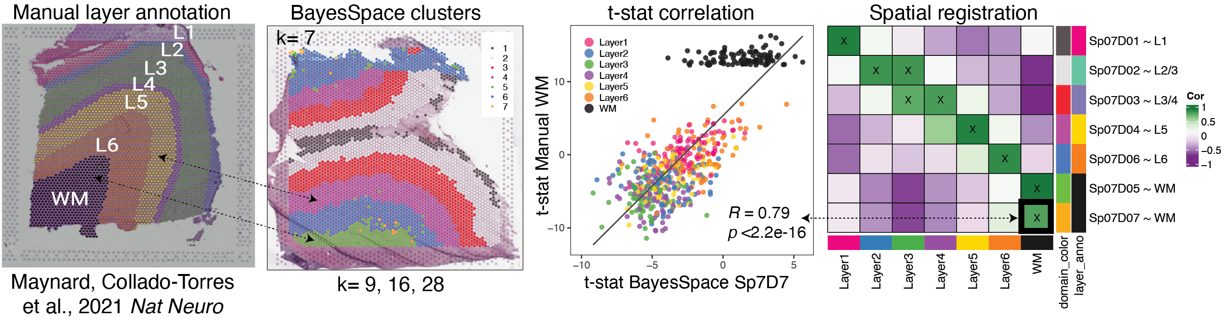
# How to run Spatial Registration with `spatialLIBD` tools

## Introduction. 

In this example we will utilize the human DLPFC 10x Genomics Visium dataset
from Maynard, Collado-Torres et al. `r Citep(bib[['spatialLIBDpaper']])` as the **reference**.
This data contains manually annotated features: the **six cortical layers + white matter**
present in the DLPFC. We will use the pre-calculated enrichment statistics for the
layers, which are available from `r Biocpkg("spatialLIBD")`.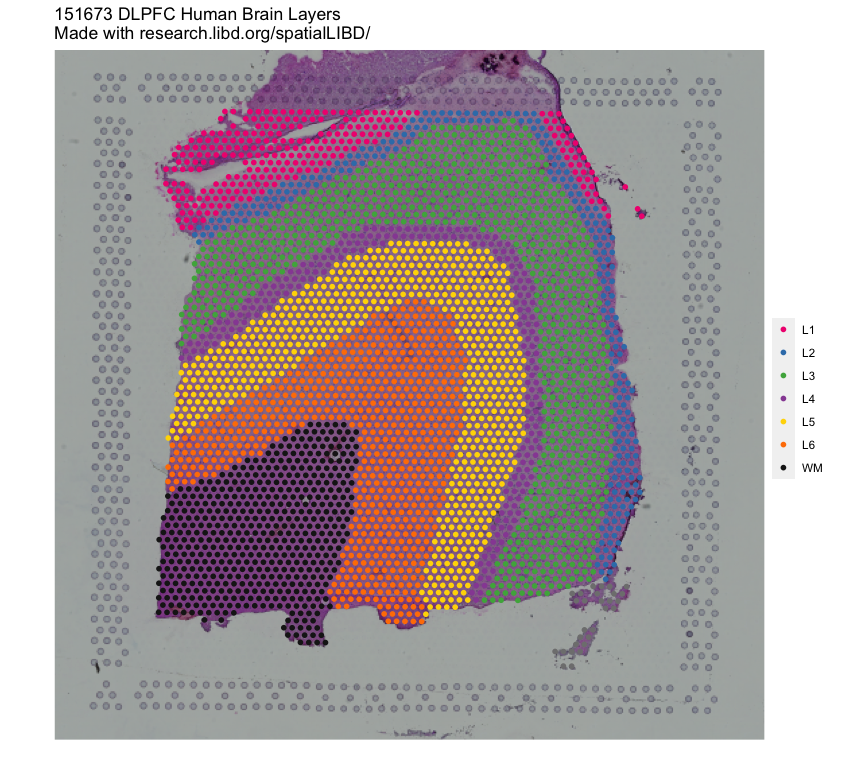

<p align="center">

![Dotplot of sample from refernce DLPFC data, colored by annotated layers](http://research.libd.org/spatialLIBD/reference/figures/README-access_data-1.png){width=100%}
</p>


The **query** dataset will be the DLPFC single nucleus RNA-seq (snRNA-seq) data from `r Citep(bib[['tran2021']])`. 

We will compare the gene expression in the cell type populations of the **query**
dataset to the annotated **layers** in the **reference**. 



## Important Notes 

### Required knowledge

It may be helpful to review _Introduction to spatialLIBD_ vignette available through [GitHub](http://research.libd.org/spatialLIBD/articles/spatialLIBD.html) or [Bioconductor](https://bioconductor.org/packages/spatialLIBD) for more information about this data set and R package. 


### Citing `spatialLIBD`

We hope that `r Biocpkg("spatialLIBD")` will be useful for your research. Please use the following information to cite the package and the overall approach. Thank you!

```{r "citation"}
## Citation info
citation("spatialLIBD")
```

## Setup 

### Install `spatialLIBD`

```{r "install", eval = FALSE}
if (!requireNamespace("BiocManager", quietly = TRUE)) {
    install.packages("BiocManager")
}

BiocManager::install("spatialLIBD")

## Check that you have a valid Bioconductor installation
BiocManager::valid()
```

### Load required packages

```{r "start", message=FALSE}
library("spatialLIBD")
library("SingleCellExperiment")
```

## Download Data

### Spatial Reference

The reference data is easily accessed through `r Biocpkg("spatialLIBD")`. The modeling results
for the annotated layers is already calculated and can be accessed with the `fetch_data()` function.

This data contains the results form three models (anova, enrichment, and pairwise),
we will use the **enrichment** results for spatial registration. The tables contain the
$t$-statistics, p-values, and gene ensembl ID and symbol. 

```{r "fetch_refrence"}
## get reference layer enrichment statistics
layer_modeling_results <- fetch_data(type = "modeling_results")

layer_modeling_results$enrichment[1:5, 1:5]
```


### Query Data: snRNA-seq 

For the query data set, we will use the public single nucleus RNA-seq (snRNA-seq) 
data from `r Citep(bib[['tran2021']])` can be accessed on [github](https://github.com/LieberInstitute/10xPilot_snRNAseq-human#processed-data).

This data is also from postmortem human brain DLPFC, and contains gene 
expression data for 11k nuclei and 19 cell types.

We will use `BiocFileCache()` to cache this data. It is stored as a `SingleCellExperiment` 
object named `sce.dlpfc.tran`, and takes 1.01 GB of RAM memory to load.  

```{r "download_sce_data"}
# Download and save a local cache of the data available at:
# https://github.com/LieberInstitute/10xPilot_snRNAseq-human#processed-data
bfc <- BiocFileCache::BiocFileCache()
url <- paste0(
    "https://libd-snrnaseq-pilot.s3.us-east-2.amazonaws.com/",
    "SCE_DLPFC-n3_tran-etal.rda"
)
local_data <- BiocFileCache::bfcrpath(url, x = bfc)

load(local_data, verbose = TRUE)
```


DLPFC tissue consists of many cell types, some are quite rare and will not have enough data to complete the analysis

```{r "check_cell_types"}
table(sce.dlpfc.tran$cellType)
```

The data will be pseudo-bulked over `donor` x `cellType`, it is recommended to drop
groups with < 10 nuclei (this is done automatically in the pseudobulk step).

```{r "donor_x_cellType"}
table(sce.dlpfc.tran$donor, sce.dlpfc.tran$cellType)
```


## Get Enrichment statistics for snRNA-seq data

`spatialLIBD` contains many functions to compute `modeling_results` for the query sc/snRNA-seq or spatial data. 

**The process includes the following steps**

1. `registration_pseudobulk()`: Pseudo-bulks data, filter low expressed genes, and normalize counts
2. `registration_mod()`: Defines the statistical model that will be used for computing the block correlation
3. `registration_block_cor()` : Computes the block correlation using the sample ID as the blocking factor, used as correlation in eBayes call
2. `registration_stats_enrichment()` : Computes the gene enrichment $t$-statistics (one group vs. All other groups)

The function `registration_wrapper()` makes life easy by wrapping these functions together in to one step!

```{r "run_registration_wrapper"}
## Perform the spatial registration
sce_modeling_results <- registration_wrapper(
    sce = sce.dlpfc.tran,
    var_registration = "cellType",
    var_sample_id = "donor",
    gene_ensembl = "gene_id",
    gene_name = "gene_name"
)
```

## Extract Enrichment t-statistics
```{r "extract_t_stats"}
## extract t-statics and rename
registration_t_stats <- sce_modeling_results$enrichment[, grep("^t_stat", colnames(sce_modeling_results$enrichment))]
colnames(registration_t_stats) <- gsub("^t_stat_", "", colnames(registration_t_stats))

## cell types x gene
dim(registration_t_stats)

## check out table
registration_t_stats[1:5, 1:5]
```


## Correlate statsics with Layer Reference

```{r "layer_stat_cor"}
cor_layer <- layer_stat_cor(
    stats = registration_t_stats,
    modeling_results = layer_modeling_results,
    model_type = "enrichment",
    top_n = 100
)

cor_layer
```

# Explore Results

Now we can use these correlation values to learn about the cell types. 

## Create Heatmap of Correlations

We can see from this heatmap what layers the different cell types are associated with.

* Oligo with WM 

* Astro with Layer 1 

* Excitatory neurons to different layers of the cortex

* Weak associate with Inhibitory Neurons


```{r layer_cor_plot}
layer_stat_cor_plot(cor_layer, max = max(cor_layer))
```

## Annotate Cell Types by Top Correlation

We can use `annotate_registered_clusters` to create annotation labels for the 
cell types based on the correlation values. 

```{r "annotate"}
anno <- annotate_registered_clusters(
    cor_stats_layer = cor_layer,
    confidence_threshold = 0.25,
    cutoff_merge_ratio = 0.25
)

anno
```


# Reproducibility

The `r Biocpkg("spatialLIBD")` package `r Citep(bib[["spatialLIBD"]])` was made possible thanks to:

* R `r Citep(bib[["R"]])`
* `r Biocpkg("BiocStyle")` `r Citep(bib[["BiocStyle"]])`
* `r CRANpkg("knitr")` `r Citep(bib[["knitr"]])`
* `r CRANpkg("RefManageR")` `r Citep(bib[["RefManageR"]])`
* `r CRANpkg("rmarkdown")` `r Citep(bib[["rmarkdown"]])`
* `r CRANpkg("sessioninfo")` `r Citep(bib[["sessioninfo"]])`
* `r CRANpkg("testthat")` `r Citep(bib[["testthat"]])`

This package was developed using `r BiocStyle::Biocpkg("biocthis")`.


Code for creating the vignette

```{r createVignette, eval=FALSE}
## Create the vignette
library("rmarkdown")
system.time(render("guide_to_spatial_registration.Rmd", "BiocStyle::html_document"))

## Extract the R code
library("knitr")
knit("guide_to_spatial_registration.Rmd", tangle = TRUE)
```

Date the vignette was generated.

```{r reproduce1, echo=FALSE}
## Date the vignette was generated
Sys.time()
```

Wallclock time spent generating the vignette.

```{r reproduce2, echo=FALSE}
## Processing time in seconds
totalTime <- diff(c(startTime, Sys.time()))
round(totalTime, digits = 3)
```

`R` session information.

```{r reproduce3, echo=FALSE}
## Session info
library("sessioninfo")
options(width = 120)
session_info()
```



# Bibliography

This vignette was generated using `r Biocpkg("BiocStyle")` `r Citep(bib[["BiocStyle"]])`
with `r CRANpkg("knitr")` `r Citep(bib[["knitr"]])` and `r CRANpkg("rmarkdown")` `r Citep(bib[["rmarkdown"]])` running behind the scenes.

Citations made with `r CRANpkg("RefManageR")` `r Citep(bib[["RefManageR"]])`.

```{r vignetteBiblio, results = "asis", echo = FALSE, warning = FALSE, message = FALSE}
## Print bibliography
PrintBibliography(bib, .opts = list(hyperlink = "to.doc", style = "html"))
```